Deep Learning

Learning outcomes

From this module, you will be able to

Explain the role of neural networks in machine learning, including their advantages and disadvantages.
Discuss why traditional methods are less effective for image data.
Gain a high-level understanding of transfer learning.
Differentiate between image classification and object detection.

Image classification

Have you used search in Google Photos? You can search for “my photos of cat” and it will retrieve photos from your libraries containing cats. This can be done using image classification, which is treated as a supervised learning problem, where we define a set of target classes (objects to identify in images), and train a model to recognize them using labeled example photos.

Image classification

Image classification is not an easy problem because of the variations in the location of the object, lighting, background, camera angle, camera focus etc.

Neural networks

Neural networks are perfect for these types of problems where local structures are important.
A significant advancement in image classification was the application of convolutional neural networks (ConvNets or CNNs) to this problem.
ImageNet Classification with Deep Convolutional Neural Networks
Achieved a winning test error rate of 15.3%, compared to 26.2% achieved by the second-best entry in the ILSVRC-2012 competition.
Let’s go over the basics of a neural network.

Introduction to neural networks

Neural networks can be viewed a generalization of linear models where we apply a series of transformations.
Here is graphical representation of a logistic regression model.
We have 4 features: x[0], x[1], x[2], x[3]

Adding a layer of transformations

Below we are adding one “layer” of transformations in between features and the target.
We are repeating the the process of computing the weighted sum multiple times.
The hidden units (e.g., h[1], h[2], …) represent the intermediate processing steps.

One more layer of transformations

Now we are adding one more layer of transformations.

Neural networks

With a neural net, you specify the number of features after each transformation.
- In the above, it goes from 4 to 3 to 3 to 1.
To make them really powerful compared to the linear models, we apply a non-linear function to the weighted sum for each hidden node.
Neural network = neural net
Deep learning ~ using neural networks

Why neural networks?

They can learn very complex functions.
- The fundamental tradeoff is primarily controlled by the number of layers and layer sizes.
- More layers / bigger layers –> more complex model.
- You can generally get a model that will not underfit.
The work really well for structured data:
- 1D sequence, e.g. timeseries, language
- 2D image
- 3D image or video
They’ve had some incredible successes in the last 10 years.
Transfer learning (coming later today) is really useful.

Why not neural networks?

Often they require a lot of data.
They require a lot of compute time, and, to be faster, specialized hardware called GPUs.
They have huge numbers of hyperparameters are a huge pain to tune.
- Think of each layer having hyperparameters, plus some overall hyperparameters.
- Being slow compounds this problem.
They are not interpretable.
I don’t recommend training them on your own without further training
- Good news
  - You don’t have to train your models from scratch in order to use them.
  - I’ll show you some ways to use neural networks without training them yourselves.

Deep learning software

The current big players are:

Both are heavily used in industry. If interested, see comparison of deep learning software.

Introduction to computer vision

Computer vision refers to understanding images/videos, usually using ML/AI.
In the last decade this field has been dominated by deep learning. We will explore image classification and object detection.

Introduction to computer vision

image classification: is this a cat or a dog?
object localization: where is the cat in this image?
object detection: What are the various objects in the image?
instance segmentation: What are the shapes of these various objects in the image?
and much more…

Pre-trained models

In practice, very few people train an entire CNN from scratch because it requires a large dataset, powerful computers, and a huge amount of human effort to train the model.
Instead, a common practice is to download a pre-trained model and fine tune it for your task. This is called transfer learning.
Transfer learning is one of the most common techniques used in the context of computer vision and natural language processing.
It refers to using a model already trained on one task as a starting point for learning to perform another task

Pre-trained models out-of-the-box

Let’s first apply one of these pre-trained models to our own problem right out of the box.

Pre-trained models out-of-the-box

We can easily download famous models using the torchvision.models module. All models are available with pre-trained weights (based on ImageNet’s 224 x 224 images)
We used a pre-trained model vgg16 which is trained on the ImageNet data.
We preprocess the given image.
We get prediction from this pre-trained model on a given image along with prediction probabilities.
For a given image, this model will spit out one of the 1000 classes from ImageNet.

Pre-trained models out-of-the-box

Let’s predict labels with associated probabilities for unseen images

                         Class  Probability score
                     tiger cat              0.353
              tabby, tabby cat              0.207
               lynx, catamount              0.050
Pembroke, Pembroke Welsh corgi              0.046
--------------------------------------------------------------

                                     Class  Probability score
         cheetah, chetah, Acinonyx jubatus              0.983
                  leopard, Panthera pardus              0.012
jaguar, panther, Panthera onca, Felis onca              0.004
       snow leopard, ounce, Panthera uncia              0.001
--------------------------------------------------------------

                                   Class  Probability score
                                 macaque              0.714
patas, hussar monkey, Erythrocebus patas              0.122
      proboscis monkey, Nasalis larvatus              0.098
                   guenon, guenon monkey              0.017
--------------------------------------------------------------

                        Class  Probability score
Walker hound, Walker foxhound              0.580
             English foxhound              0.091
                  EntleBucher              0.080
                       beagle              0.065
--------------------------------------------------------------

Pre-trained models out-of-the-box

We got these predictions without “doing the ML ourselves”.
We are using pre-trained vgg16 model which is available in torchvision.
- torchvision has many such pre-trained models available that have been very successful across a wide range of tasks: AlexNet, VGG, ResNet, Inception, MobileNet, etc.
Many of these models have been pre-trained on famous datasets like ImageNet.
So if we use them out-of-the-box, they will give us one of the ImageNet classes as classification.

Pre-trained models out-of-the-box

Let’s try some images which are unlikely to be there in ImageNet.
It’s not doing very well here because ImageNet doesn’t have proper classes for these images.

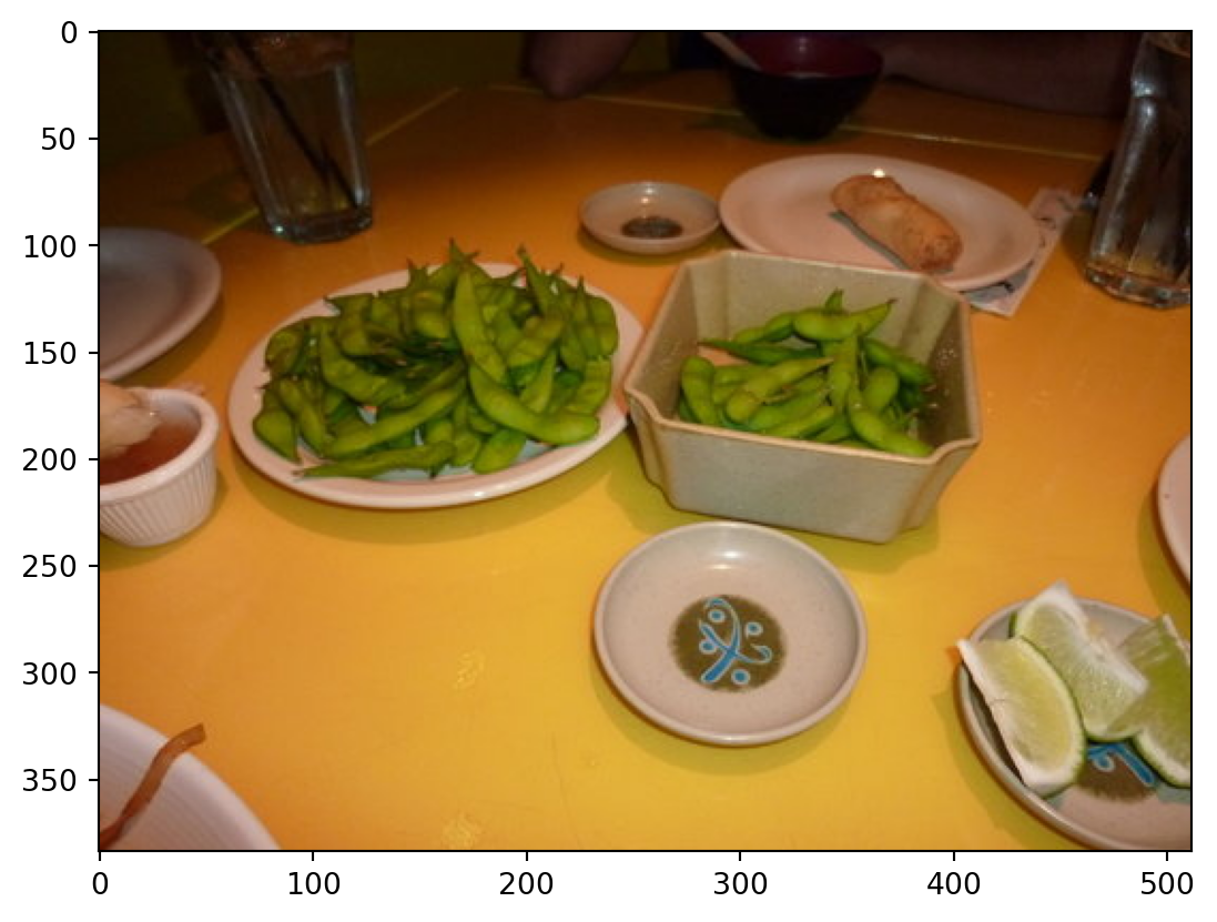
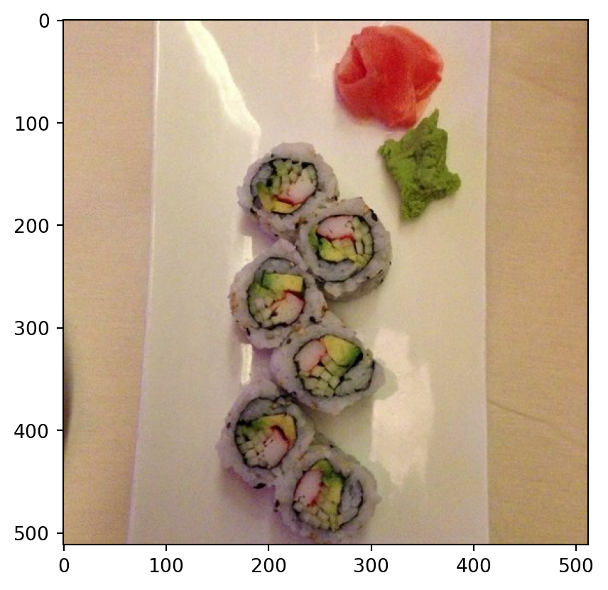
         Class  Probability score
cucumber, cuke              0.146
         plate              0.117
     guacamole              0.099
  Granny Smith              0.091
--------------------------------------------------------------

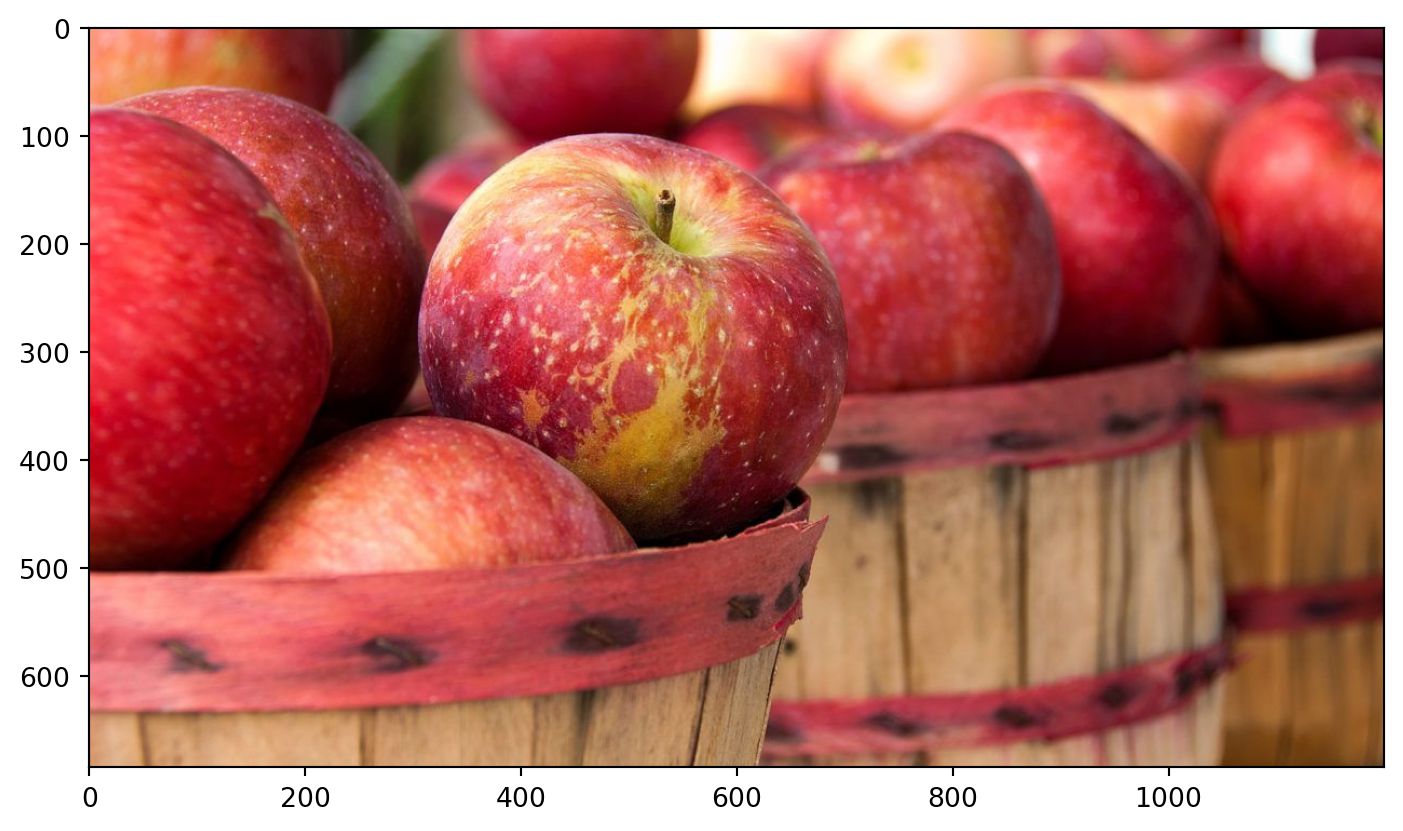
                                      Class  Probability score
                                        fig              0.637
                                pomegranate              0.193
grocery store, grocery, food market, market              0.041
                                      crate              0.023
--------------------------------------------------------------

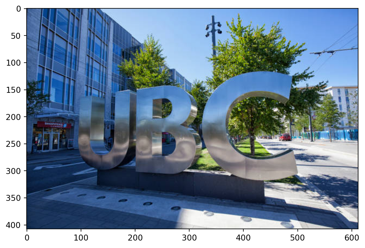
                                               Class  Probability score
                                         toilet seat              0.171
                                          safety pin              0.060
bannister, banister, balustrade, balusters, handrail              0.039
                                              bubble              0.035
--------------------------------------------------------------

                  Class  Probability score
                   vase              0.078
                thimble              0.074
             plate rack              0.049
saltshaker, salt shaker              0.047
--------------------------------------------------------------

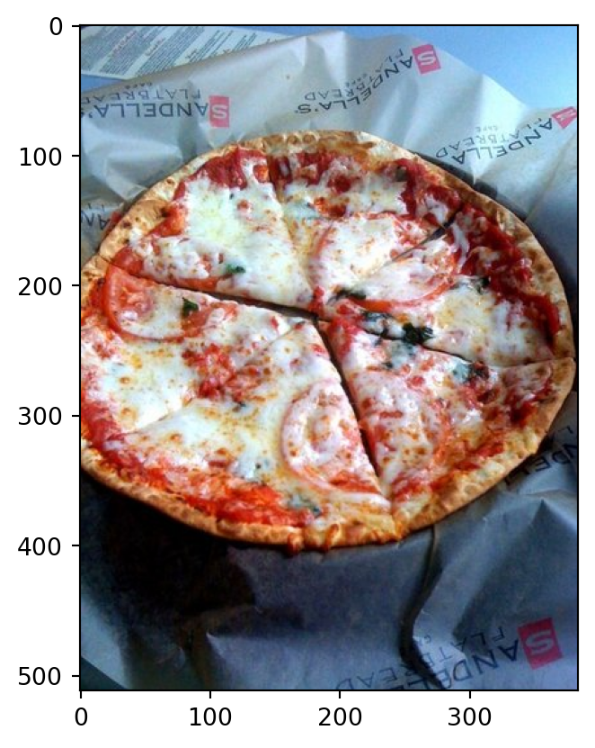
                      Class  Probability score
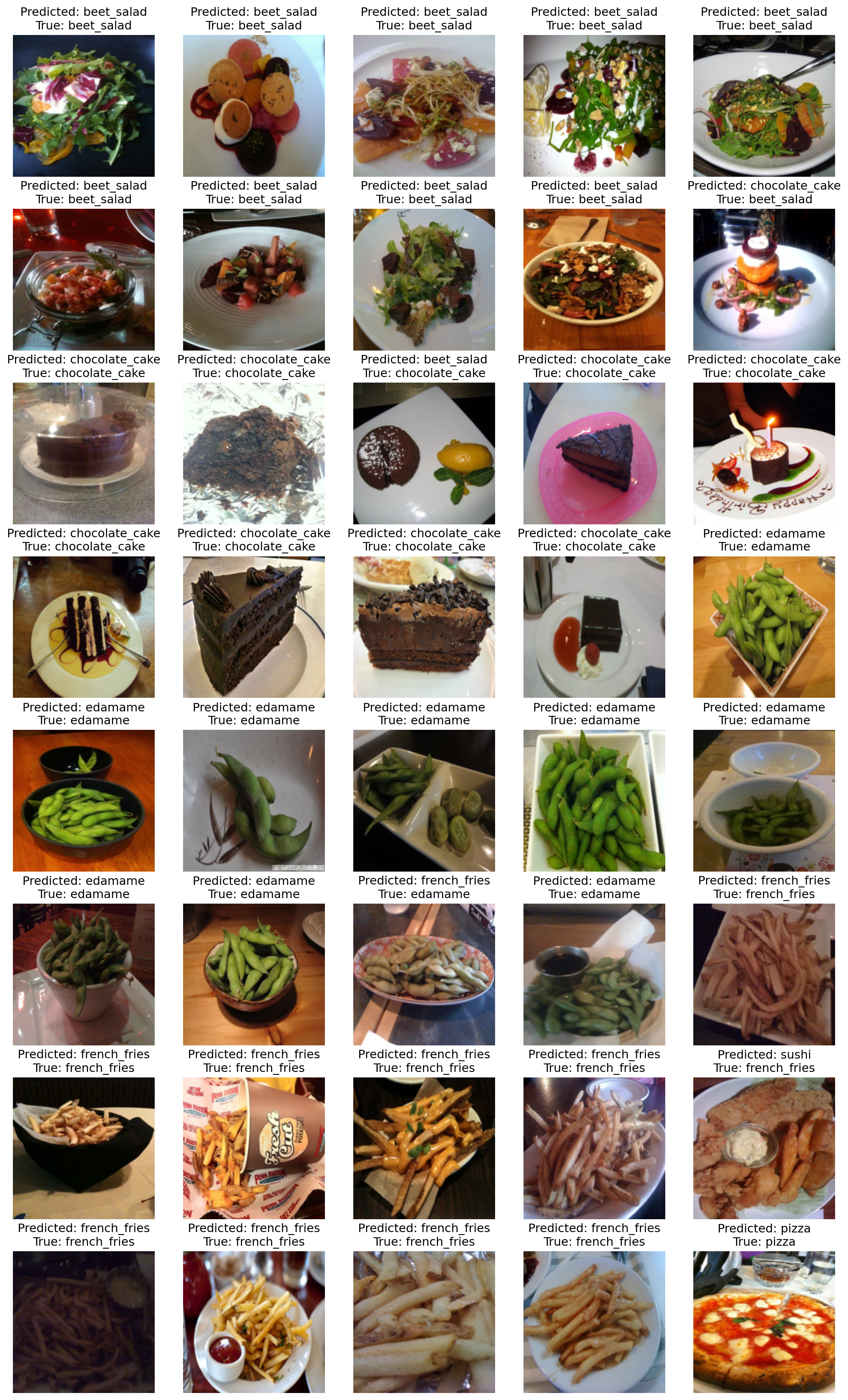
           pizza, pizza pie              0.998
frying pan, frypan, skillet              0.001
                     potpie              0.000
                French loaf              0.000
--------------------------------------------------------------

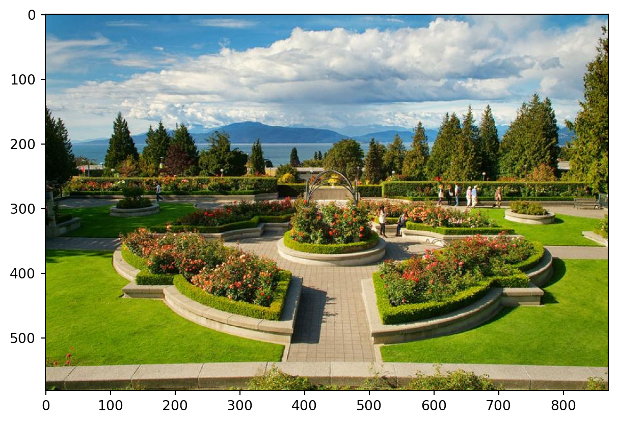
              Class  Probability score
     patio, terrace              0.213
           fountain              0.164
lakeside, lakeshore              0.097
            sundial              0.088
--------------------------------------------------------------

Pre-trained models out-of-the-box

Here we are Pre-trained models out-of-the-box.
Can we use pre-trained models for our own classification problem with our classes?
Yes!! We have two options here:
1. Add some extra layers to the pre-trained network to suit our particular task
2. Pass training data through the network and save the output to use as features for training some other model

Pre-trained models to extract features

Let’s use pre-trained models to extract features.
We will pass our specific data through a pre-trained network to get a feature vector for each example in the data.
The feature vector is usually extracted from the last layer, before the classification layer from the pre-trained network.
You can think of each layer a transformer applying some transformations on the input received to that later.

Pre-trained models to extract features

Once we extract these feature vectors for all images in our training data, we can train a machine learning classifier such as logistic regression or random forest.
This classifier will be trained on our classes using feature representations extracted from the pre-trained models.
Let’s try this out.
It’s better to train such models with GPU. Since our dataset is quite small, we won’t have problems running it on a CPU.

Pre-trained models to extract features

Let’s look at some sample images in the dataset.

Dataset statistics

Here is the stat of our toy dataset.

Classes: ['beet_salad', 'chocolate_cake', 'edamame', 'french_fries', 'pizza', 'spring_rolls', 'sushi']
Class count: 40, 38, 40
Samples: 283
First sample: ('data/food/train/beet_salad/104294.jpg', 0)

Pre-trained models to extract features

Now for each image in our dataset, we’ll extract a feature vector from a pre-trained model called densenet121, which is trained on the ImageNet dataset.

Shape of the feature vector

Now we have extracted feature vectors for all examples. What’s the shape of these features?

torch.Size([283, 1024])

The size of each feature vector is 1024 because the size of the last layer in densenet architecture is 1024.

Source

A feature vector given by densenet

Let’s examine the feature vectors.

	0	1	2	3	4	5	6	7	8	9	...	1014	1015	1016	1017	1018	1019	1020	1021	1022	1023
0	0.000290	0.003821	0.005015	0.001307	0.052690	0.063403	0.000626	0.001850	0.256254	0.000223	...	0.229936	1.046364	2.241251	0.229642	0.033676	0.742794	1.338703	2.130873	0.625468	0.463095
1	0.000407	0.005973	0.003206	0.001932	0.090702	0.438522	0.001513	0.003906	0.166081	0.000286	...	0.910675	1.580823	0.087190	0.606906	0.436105	0.306454	0.940104	1.159830	1.712701	1.624746
2	0.000626	0.005090	0.002887	0.001299	0.091715	0.548536	0.000491	0.003587	0.266537	0.000408	...	0.465154	0.678282	0.946386	1.194696	2.537741	1.642386	0.701204	0.115618	0.186435	0.166608
3	0.000169	0.006087	0.002489	0.002167	0.087537	0.623212	0.000427	0.000226	0.460680	0.000388	...	0.394087	0.700154	0.105199	0.856322	0.038457	0.023949	0.131834	1.296366	0.723329	1.915226
4	0.000286	0.005520	0.001906	0.001599	0.186035	0.850148	0.000835	0.003025	0.036309	0.000142	...	3.313759	0.565747	0.473564	0.139445	0.029284	1.165939	0.442323	0.227595	0.884269	1.592694

5 rows × 1024 columns

The features are hard to interpret but they have some important information about the images which can be useful for classification.

Logistic regression with the extracted features

Let’s try out logistic regression on these extracted features.

Training score:  1.0

Validation score:  0.835820895522388

This is great accuracy for so little data and little effort!!!

Sample predictions

Let’s examine some sample predictions on the validation set.

Object detection

Another useful task and tool to know is object detection using YOLO model.
Let’s identify objects in a sample image using a pretrained model called YOLO8.
List the objects present in this image.

Object detection using YOLO

Let’s try this out using a pre-trained model.

from ultralytics import YOLO
model = YOLO("yolov8n.pt")  # pretrained YOLOv8n model

yolo_input = "data/yolo_test/3356700488_183566145b.jpg"
yolo_result = "data/yolo_result.jpg"
# Run batched inference on a list of images
result = model(yolo_input)  # return a list of Results objects
result[0].save(filename=yolo_result)

image 1/1 /Users/kvarada/EL/workshops/DSI-ML-workshop-2024/website/slides/data/yolo_test/3356700488_183566145b.jpg: 512x640 4 persons, 2 cars, 1 stop sign, 259.3ms
Speed: 3.6ms preprocess, 259.3ms inference, 8.0ms postprocess per image at shape (1, 3, 512, 640)

'data/yolo_result.jpg'

Object detection output

Summary

Neural networks are a flexible class of models.
- They are particular powerful for structured input like images, videos, audio, etc.
- They can be challenging to train and often require significant computational resources.
The good news is we can use pre-trained neural networks.
- This saves us a huge amount of time/cost/effort/resources.
- We can use these pre-trained networks directly or use them as feature transformers.