Tree-based models
![]()
We have seen that decision trees are prone to overfitting. There are several models that extend the basic idea of using decision trees.
Random Forest
![]()
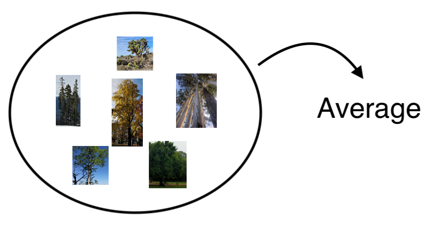
Train an ensemble of distinct decision trees.
Random Forest
Each tree trains on a random sample of the data. Some times the features used to split are also randomized at each node.
Idea: Individual trees still learn noise in the data, but the noise should “average out” over the ensemble.
Gradient Boosted Trees
![]()
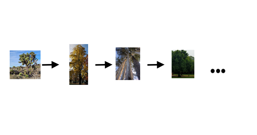
Each tree tries to “correct” or improve the previous tree’s prediction.
Tree-Based Models
Random Forest, XGBoost, etc are all easily available as “out-of-the box solutions”.
Pros:
- Perform well on a variety of tasks
- Random forest in particular are easy to train and robust to outliers.
Cons:
- Not always interpretable
- Not good at handling sparse data
- Can also still overfit.
Linear models
![]()
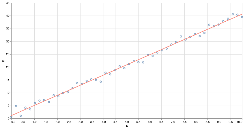
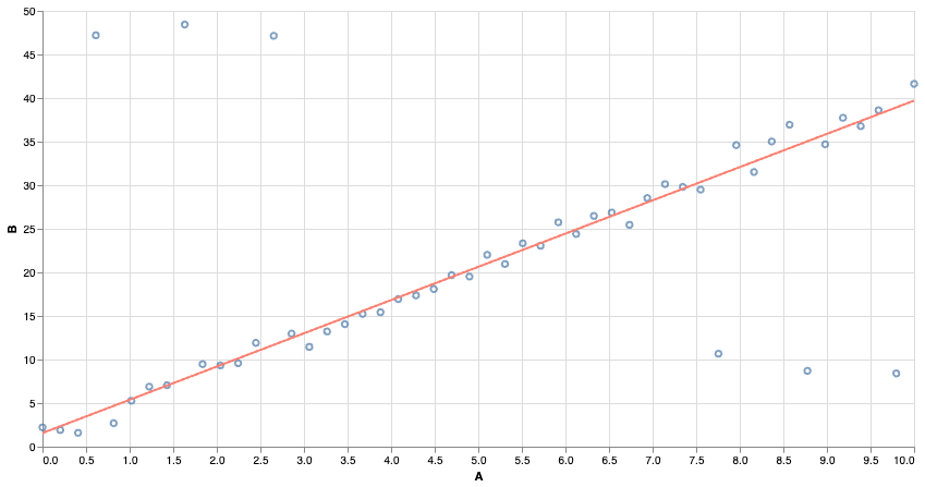
Many of you might be familiar with least-squares regression. We find the line of best fit by minimizing the ‘squared error’ of the predictions.
Linear Models
![]()
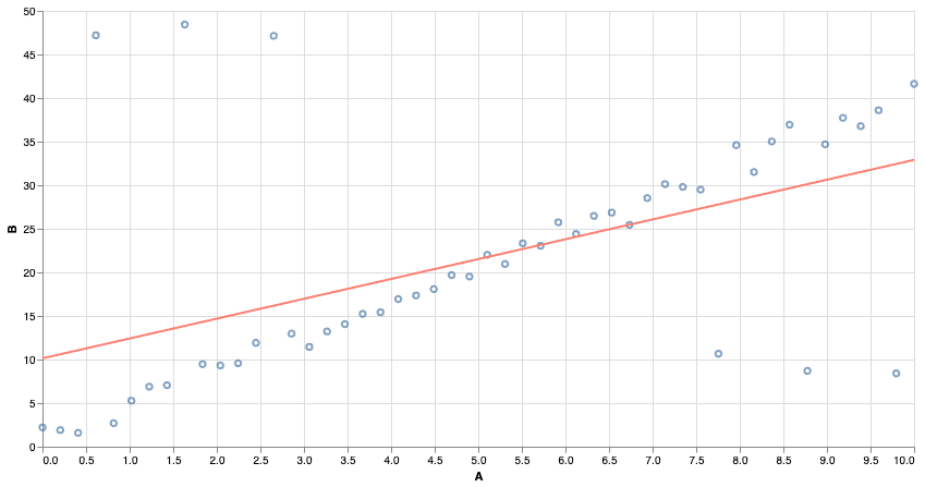
Squared Error is very sensitive to outliers. Far-away points contribute a very large squared error, and even relatively few points can affect the outcome.
Linear Models
![]()
We can use other notions of “best fit”. Using absolute error makes the model more resistant to outliers!
Linear Classifiers
We can also build linear models for classification tasks. The idea is to convert the output from an arbitrary number to a number between 0 and 1, and treat it like a “probability”.
In logistic regression, we squash the output using the sigmoid function and then adjust parameters (in training) to find the choice that makes the data “most likely”.
Linear Classifiers
![]()
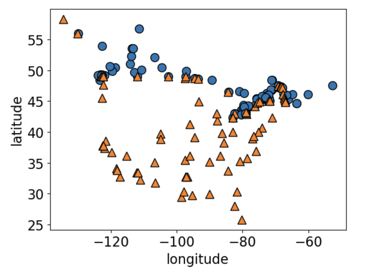
Can you guess what this dataset is?
Linear Classifiers
![]()
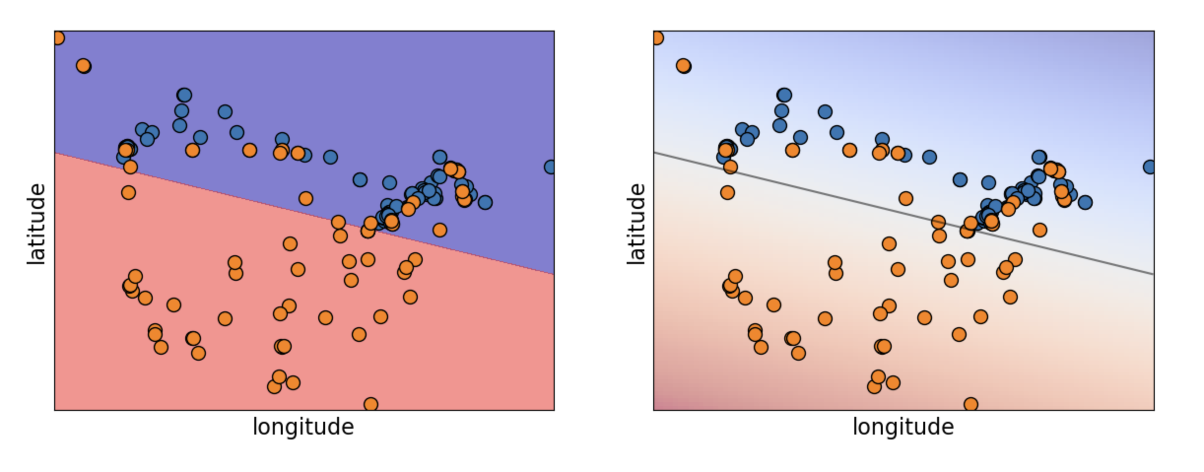
Logistic Regression predicts a linear decision boundary.
Linear Models
Pros:
- Easy to train and to interpret
- Widely applicable despite some strong assumptions
- If you have a regression task, check whether a linear regression is already good enough! If you have a classification task, logistic regression is a go-to first option.
Cons:
- Strong assumptions
- Linear decision boundaries for classifiers
- Correlated features can cause problems
Analogy and similarity in Machine Learning
Analogy-based models
![]()
Returning to our older dataset.
Analogy-based models
![]()
How would you classify the green dot?
Analogy-based models
Idea: predict on new data based on “similar” examples in the training data.
K-Nearest-Neighbour Classifier
Find the K nearest neighbours of an example, and predict whichever class was most common among them.
‘K’ is a hyperparameter. Choosing K=1 is likely to overfit. If the dataset has N examples, setting K=N just predicts the mode (dummy classifier).
No training phase, but the model can get arbitrarily large (and take very long to make predictions).
Cosine Similarity
Another popular choice for measuring similarity is “cosine distance”. Useful when orientation matters more than absolute size.
Popular choice in word embeddings when working with text data.
The RBF Kernel
The RBF kernel “transforms” our data into a representation that directly captures similarity between examples. We get a new column (i.e. new feature) for every data point. The value of the new features is determined by computing pairwise distances between points, and then applying a Gaussian.
Feature values are close to zero for far-away points, and close to 1 for nearby points.
Linear models with RBF kernel
We can train a linear model on the new features!
The model stores examples with positive and negative weights. Being close to a positive example makes your label more likely to be positive.
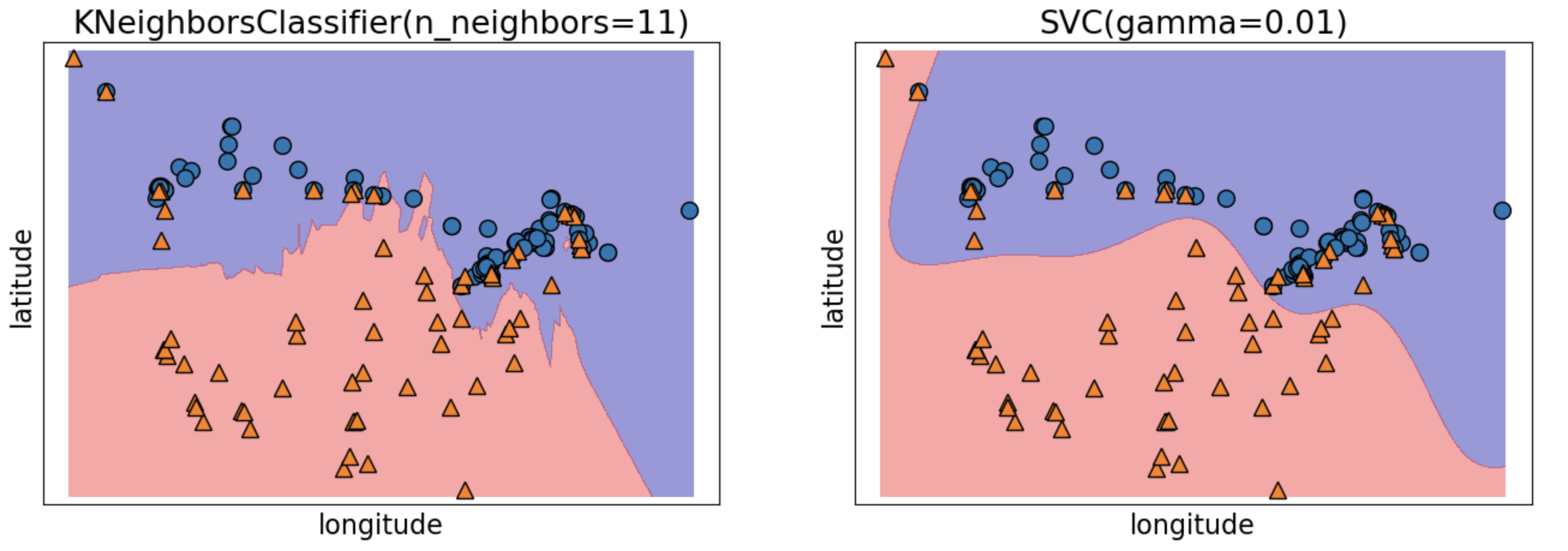
Can lead to “smoother” decision boundaries than K-NNs, and potentially to a smaller trained model.
KNNs and SVMs
![]()
Analogy-based Models
Pros:
- Do not need to make assumptions about the underlying data
- Given enough data, should pretty much always work.
Cons:
- Enough data can mean … a lot
- Computing distances is time-consuming for large datasets
- Can’t really interpret the model’s decisions.
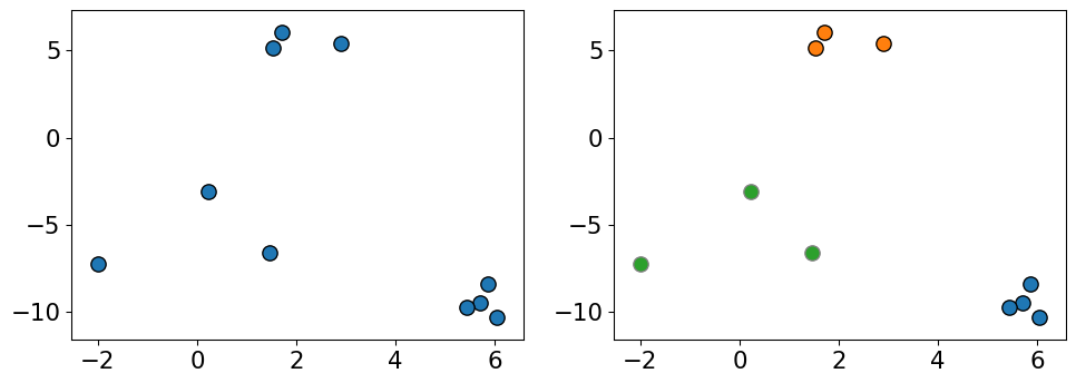
K-means clustering
![]()
K-means clustering
- Algorithm Steps: 1. Select K initial centroids. 2. Assign each data point to the nearest centroid. 3. Recalculate centroids based on assigned points. 4. Repeat until centroids stabilize or reach a maximum number of iterations.
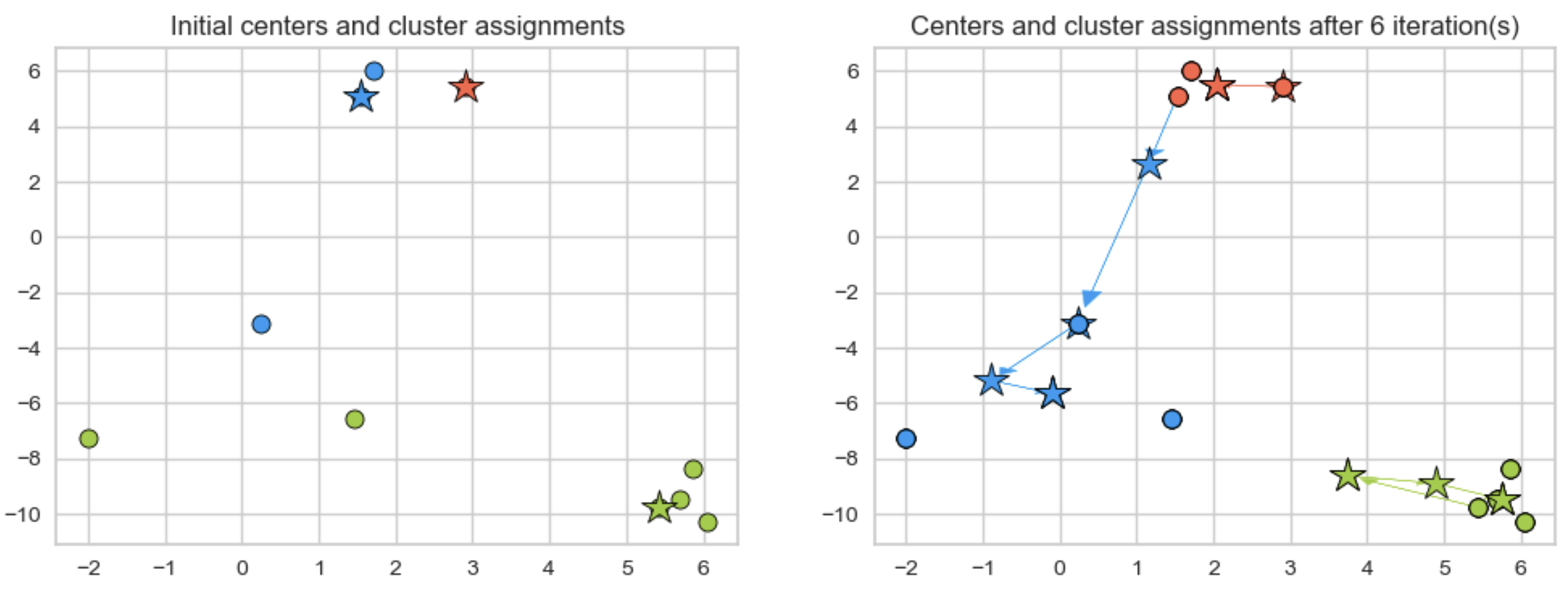
K-means clustering
![]()
K-Means pros and cons
- Advantages:
- Simple and efficient for large datasets.
- Works well with spherical clusters.
- Limitations:
- Needs pre-defined K.
- Sensitive to outliers and initial centroid placement.
- Poor performance for irregular clusters, or clusters of varying sizes and densities
Other Clustering Algorithms
Some other clustering options that offer more flexibility than K-means:
- Gaussian Mixture Models
- Density-based Clustering (DBSCAN)
- Heirarchical Clustering
Remember, data representation matters!
A Look Ahead
We saw an example of a linear model that was able to learn a non-linear decision boundary. The key was finding a non-linear feature transformation that was appropriate for the problem.
Even if our data is not linearly separable, there could be a good choice of feature transform out there that makes it linearly separable.
Wouldn’t it be nice if we could train a machine learning model to find such a transform?