Supervised Machine Learning Models

Supervised Learning

In the next section, we will briefly introduce a few types of machine learning models that are often used for supervised learning tasks.

We will discuss some basic intuition around how they work, and also discuss their relative strengths and shortcomings.

Tree-based models

We have seen that decision trees are prone to overfitting. There are several models that extend the basic idea of using decision trees.

Random Forest

Train an ensemble of distinct decision trees.

Random Forest

Each tree trains on a random sample of the data. Some times the features used to split are also randomized at each node.

Idea: Individual trees still learn noise in the data, but the noise should “average out” over the ensemble.

Gradient Boosted Trees

Each tree tries to “correct” or improve the previous tree’s prediction.

Tree-Based Models

Random Forest, XGBoost, etc are all easily available as “out-of-the box solutions”.

Pros:

Perform well on a variety of tasks
Random forest in particular are easy to train and robust to outliers.

Cons:

Not always interpretable
Not good at handling sparse data
Can also still overfit.

Linear models

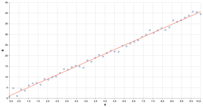
Many of you might be familiar with least-squares regression. We find the line of best fit by minimizing the ‘squared error’ of the predictions.

Linear Models

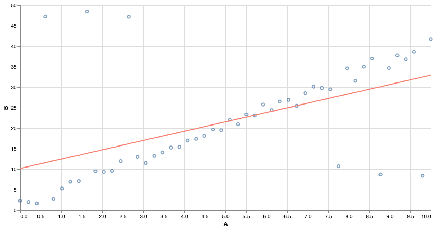
Squared Error is very sensitive to outliers. Far-away points contribute a very large squared error, and even relatively few points can affect the outcome.

Linear Models

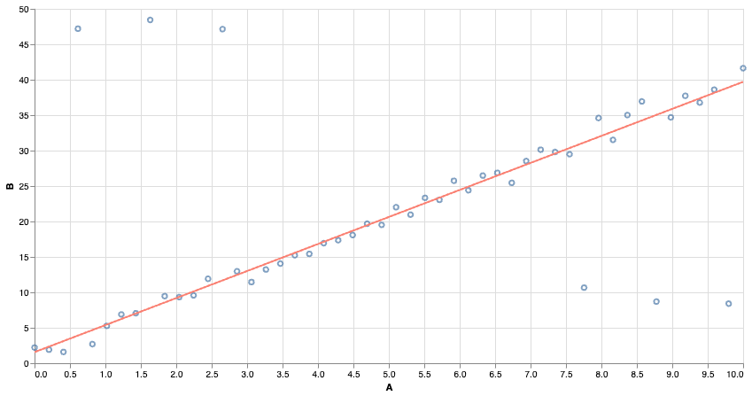
We can use other notions of “best fit”. Using absolute error makes the model more resistant to outliers!

Linear Classifiers

We can also build linear models for classification tasks. The idea is to convert the output from an arbitrary number to a number between 0 and 1, and treat it like a “probability”.

In logistic regression, we squash the output using the sigmoid function and then adjust parameters (in training) to find the choice that makes the data “most likely”.

Linear Classifiers

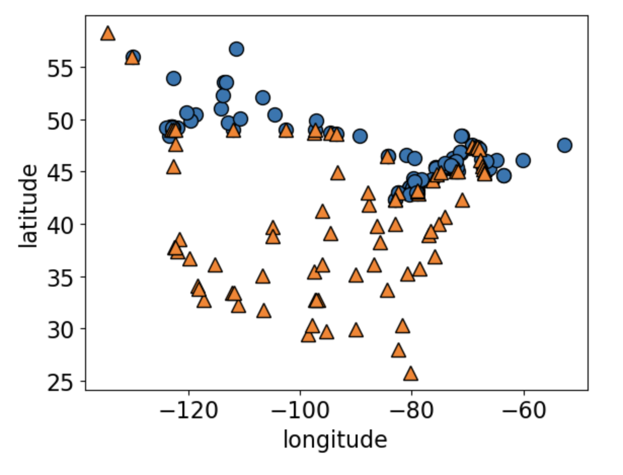
Can you guess what this dataset is?

Linear Classifiers

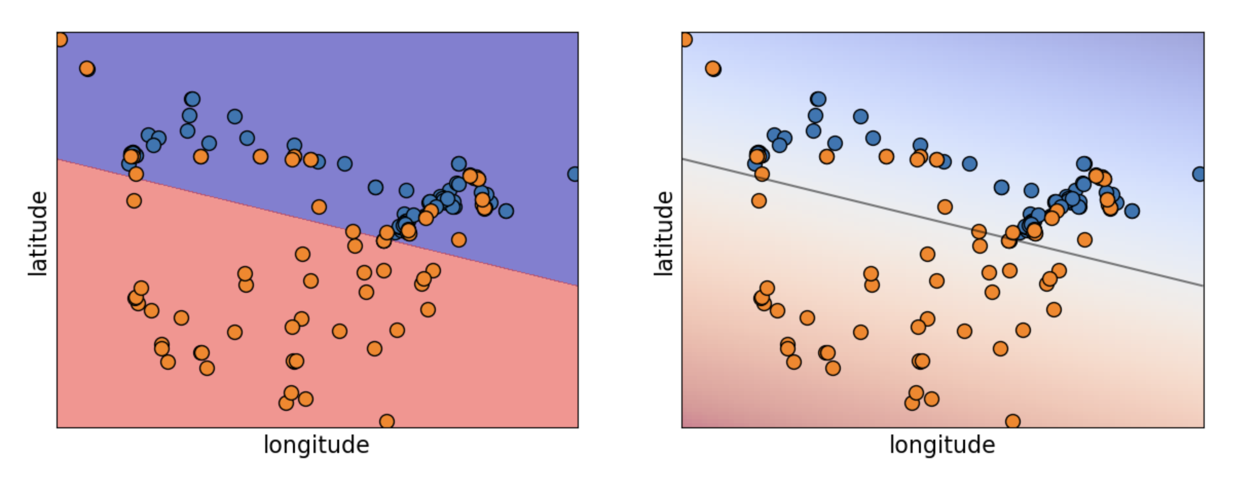
Logistic Regression predicts a linear decision boundary.

Sentiment Analysis: An Example

Let us attempt to use logistic regression to do sentiment analysis on a database of IMDB reviews. The database is available here.

imdb_df = pd.read_csv("data/imdb_master.csv", encoding="ISO-8859-1")
imdb_df.rename(columns={"sentiment": "label"}, inplace = True)

	review	label
0	One of the other reviewers has mentioned that ...	positive
1	A wonderful little production. <br /><br />The...	positive
2	I thought this was a wonderful way to spend ti...	positive
3	Basically there's a family where a little boy ...	negative
4	Petter Mattei's "Love in the Time of Money" is...	positive

We will use only about 10% of the dataset for training (to speed things up)

Bag of Words

To create features that logistic regression can use, we will represent these reviews via a “bag of words” strategy.

We create a new feature for every word that appears in the dataset. Then, if a review contains that word exactly once, the corresponding feature gets a value of 1 for that review. If the word appears four times, the feature gets a value of 4. If the word is not present, it’s marked as 0.

Bag of Words

Notice that the result is a sparse matrix. Most reviews contain only a small number of words.

vec = CountVectorizer(stop_words="english")
bow = vec.fit_transform(X_train)
bow

<Compressed Sparse Row sparse matrix of dtype 'int64'
    with 439384 stored elements and shape (5000, 38867)>

There are a total of 38867 “words” among the reviews. Here are some of them:

array(['00', 'affection', 'apprehensive', 'barbara', 'blore',
       'businessman', 'chatterjee', 'commanding', 'cramped', 'defining',
       'displaced', 'edie', 'evolving', 'fingertips', 'gaffers',
       'gravitas', 'heist', 'iliad', 'investment', 'kidnappee',
       'licentious', 'malã', 'mice', 'museum', 'obsessiveness',
       'parapsychologist', 'plasters', 'property', 'reclined',
       'ridiculous', 'sayid', 'shivers', 'sohail', 'stomaches', 'syrupy',
       'tolerance', 'unbidden', 'verneuil', 'wilcox'], dtype=object)

Checking the class counts

Let us see how many reviews are positive, and how many are negative.

y_train.value_counts()

label
positive    2517
negative    2483
Name: count, dtype: int64

The dataset looks pretty balanced, so a classifier predicting at random would at best guess about 50% correctly.

We will not train our model.

Testing Performance

Let’s see how the model performs after training.

	fit_time	score_time	test_score	train_score
0	0.411476	0.058247	0.828	0.99975
1	0.407961	0.059842	0.830	0.99975
2	0.422086	0.058663	0.848	0.99975
3	0.408087	0.057880	0.833	1.00000
4	0.397947	0.059378	0.840	0.99975

We’re able to predict with roughly 84% accuracy on validation sets. Looks like our model learned something!

Tuning hyperparameters

However, the training scores are perfect (and higher than validation scores) so our model is likely overfitting.

Maybe it just memorized some rare words, each appearing only in one review, and associated these with the review’s label. We could try reducing the size of our dictionary to prevent this.

Tuning hyperparameters

There are many tools available to automate the search for good hyperparameters. These can make our life easy, but there is always the danger of optimization bias in the results.

Investigating the model

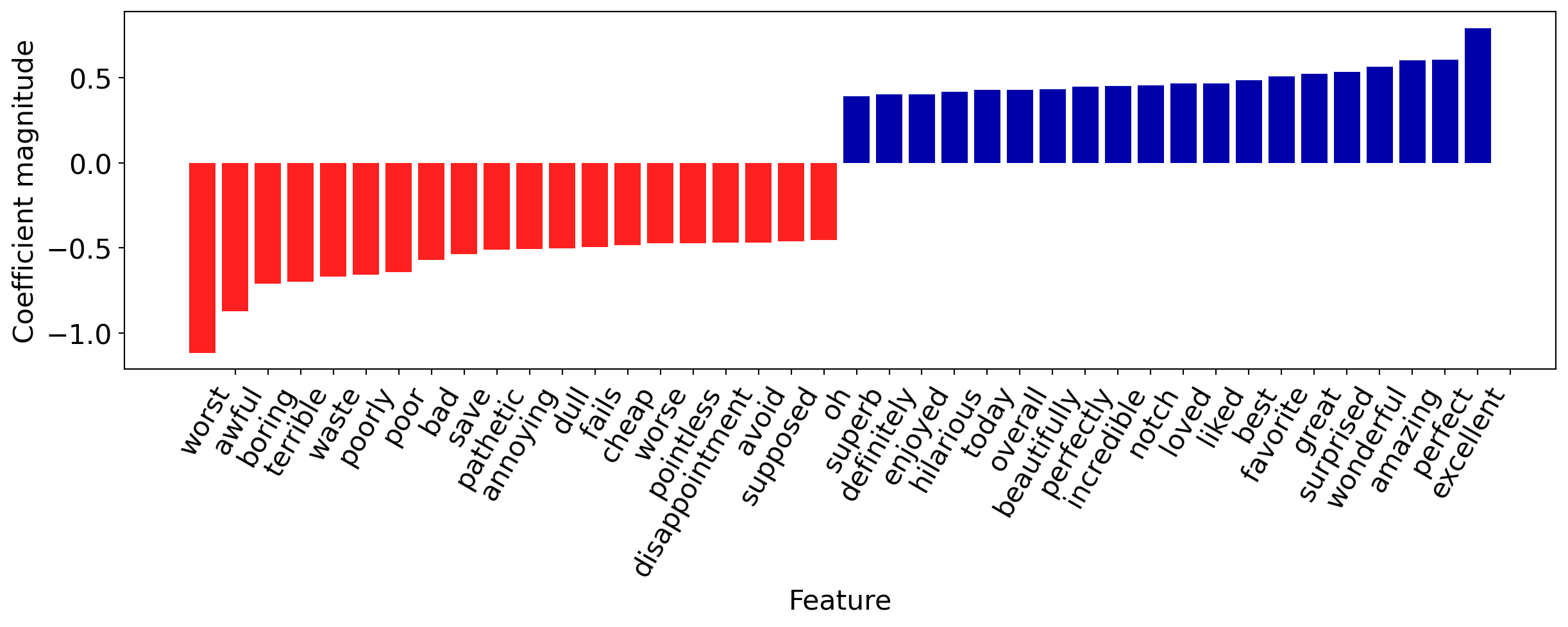
Let’s see what associations our model learned.

	Coefficient
excellent	0.792911
perfect	0.608851
amazing	0.602716
wonderful	0.564188
surprised	0.536449
...	...
waste	-0.669122
terrible	-0.697831
boring	-0.709981
awful	-0.870623
worst	-1.117365

5775 rows × 1 columns

Investigating the model

They make sense! Let’s visualize the 20 most important features.

Making Predictions

Finally, let’s try predicting on some new examples.

['It got a bit boring at times but the direction was excellent and the acting was flawless. Overall I enjoyed the movie and I highly recommend it!',
 'The plot was shallower than a kiddie pool in a drought, but hey, at least we now know emojis should stick to texting and avoid the big screen.']

Here are the model predictions:

array(['positive', 'negative'], dtype=object)

Let’s see which vocabulary words were present in the first review, and how they contributed to the classification.

Understanding Predictions

It got a bit boring at times but the direction was excellent and the acting was flawless. Overall I enjoyed the movie and I highly recommend it!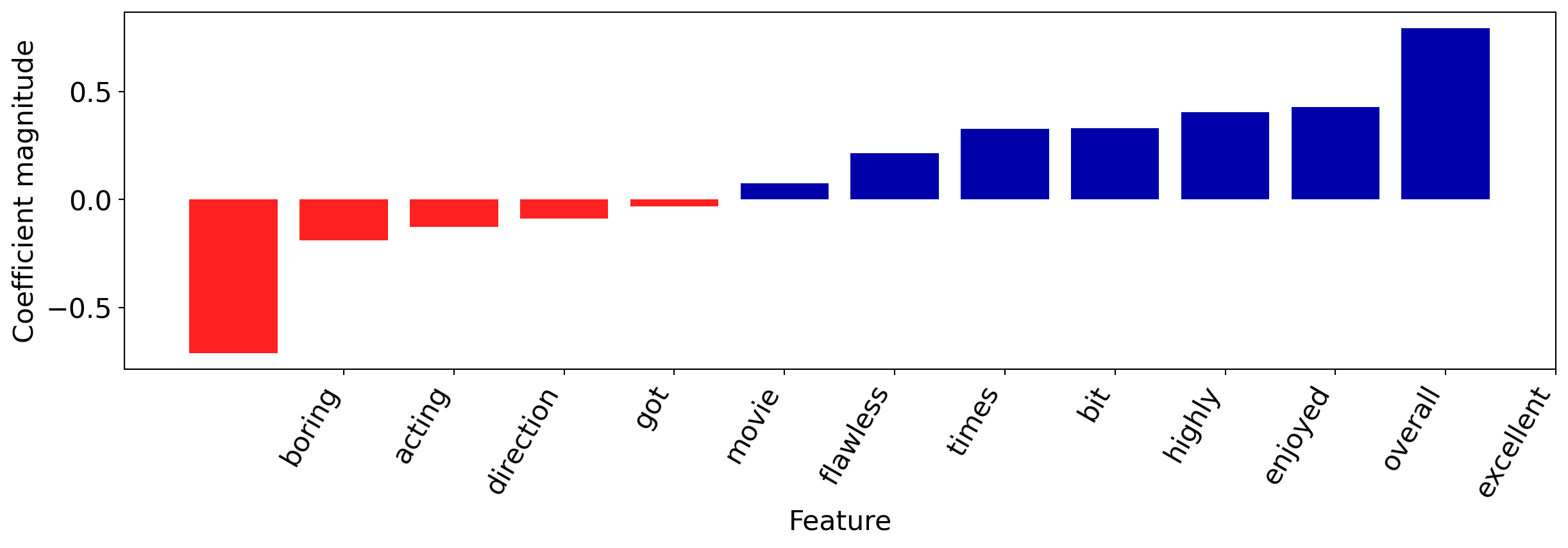

Summary

The bag-of-words representation was very simple– we only counted which words appeared in which reviews. There was no attempt to maintain syntactical or grammatical structure or to study correlations between words.

We also trained on just 5000 examples. Nevertheless, our model performs quite well.

Linear Models

Pros:

Easy to train and to interpret
Widely applicable despite some strong assumptions
If you have a regression task, check whether a linear regression is already good enough! If you have a classification task, logistic regression is a go-to first option.

Cons:

Strong assumptions
Linear decision boundaries for classifiers
Correlated features can cause problems

(Optional) Analogy-based models

Analogy-based models

Returning to our older dataset.

Analogy-based models

How would you classify the green dot?

Analogy-based models

Idea: predict on new data based on “similar” examples in the training data.

K-Nearest-Neighbour Classifier

Find the K nearest neighbours of an example, and predict whichever class was most common among them.

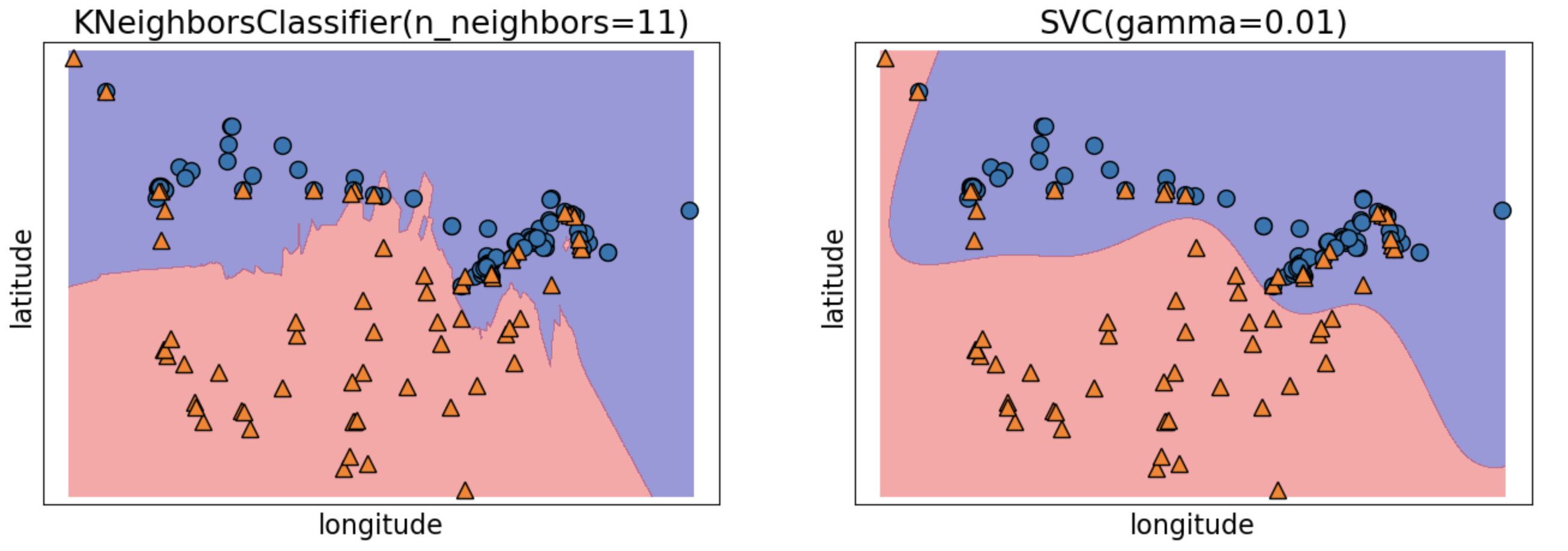
‘K’ is a hyperparameter. Choosing K=1 is likely to overfit. If the dataset has N examples, setting K=N just predicts the mode (dummy classifier).

No training phase, but the model can get arbitrarily large (and take very long to make predictions).

SVM with RBF kernel

Another ‘analogy-based’ classification method.

The model stores examples with positive and negative weights. Being close to a positive example makes your label more likely to be positive.

Can lead to “smoother” decision boundaries than K-NNs, and potentially to a smaller trained model.

KNNs and SVMs

Analogy-based Models

Pros:

Do not need to make assumptions about the underlying data
Given enough data, should pretty much always work.

Cons:

Enough data can mean … a lot
Computing distances is time-consuming for large datasets
Can’t really interpret the model’s decisions.

A Look Ahead

Support Vector Machines (SVM) are also linear classifiers.

The reason we see a non-linear decision boundary is the use of the RBF kernel, which applies a certain non-linear transformation to the features.

Even if our data is not linearly separable, there could be a good choice of feature transform out there that makes it linearly separable.

Wouldn’t it be nice if we could train a machine learning model to find such a transform?