| ml_experience | class_attendance | lab1 | lab2 | lab3 | lab4 | quiz1 | quiz2 | |
|---|---|---|---|---|---|---|---|---|
| 0 | 1 | 1 | 92 | 93 | 84 | 91 | 92 | 90 |
| 1 | 1 | 0 | 94 | 90 | 80 | 83 | 91 | 84 |
| 2 | 0 | 0 | 78 | 85 | 83 | 80 | 80 | 82 |
| 3 | 0 | 1 | 91 | 94 | 92 | 91 | 89 | 92 |
| 4 | 0 | 1 | 77 | 83 | 90 | 92 | 85 | 90 |
| 5 | 1 | 0 | 70 | 73 | 68 | 74 | 71 | 75 |
| 6 | 1 | 0 | 80 | 88 | 89 | 88 | 91 | 91 |
Introduction to Machine Learning
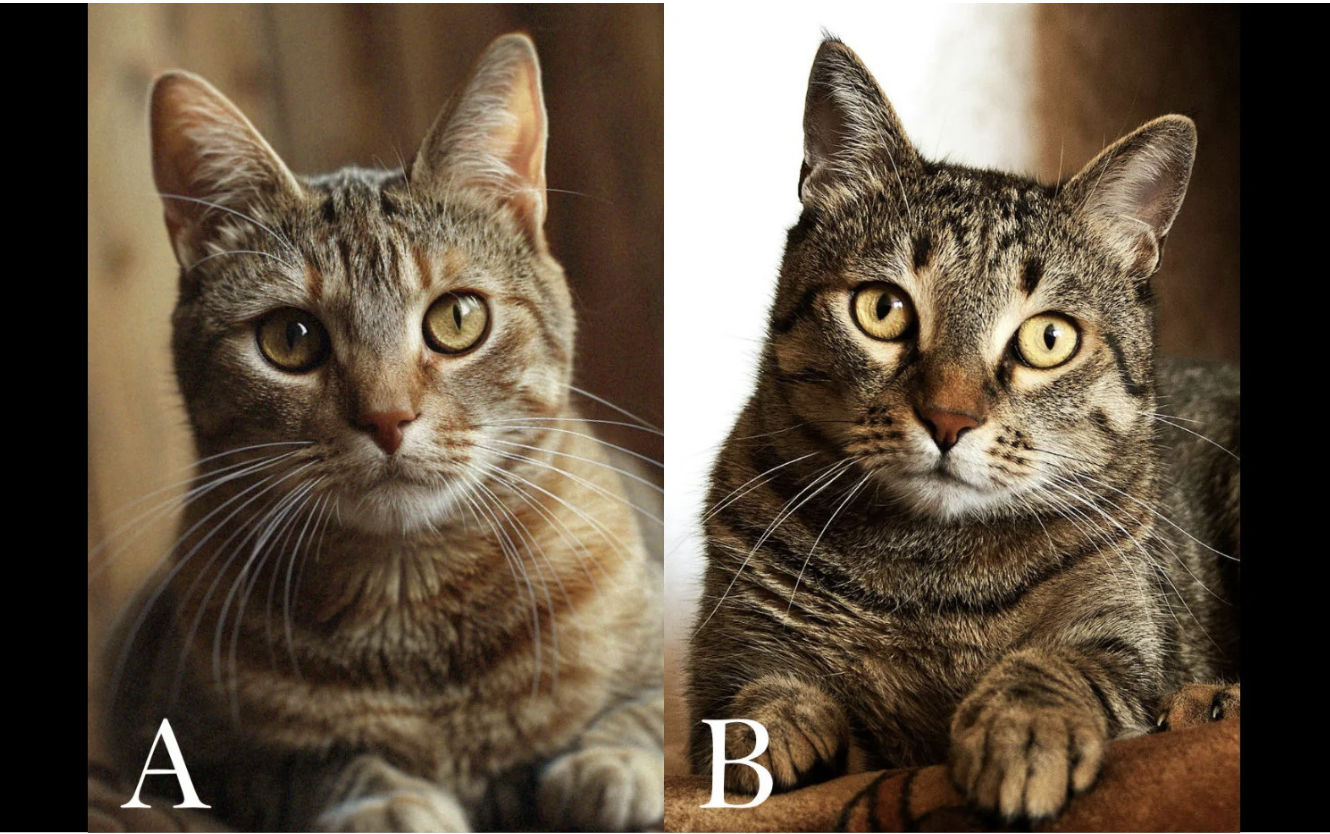
Which cat do you think is AI-generated?
 .
.
- A
- B
- Both
- None
- What clues did you use to decide?
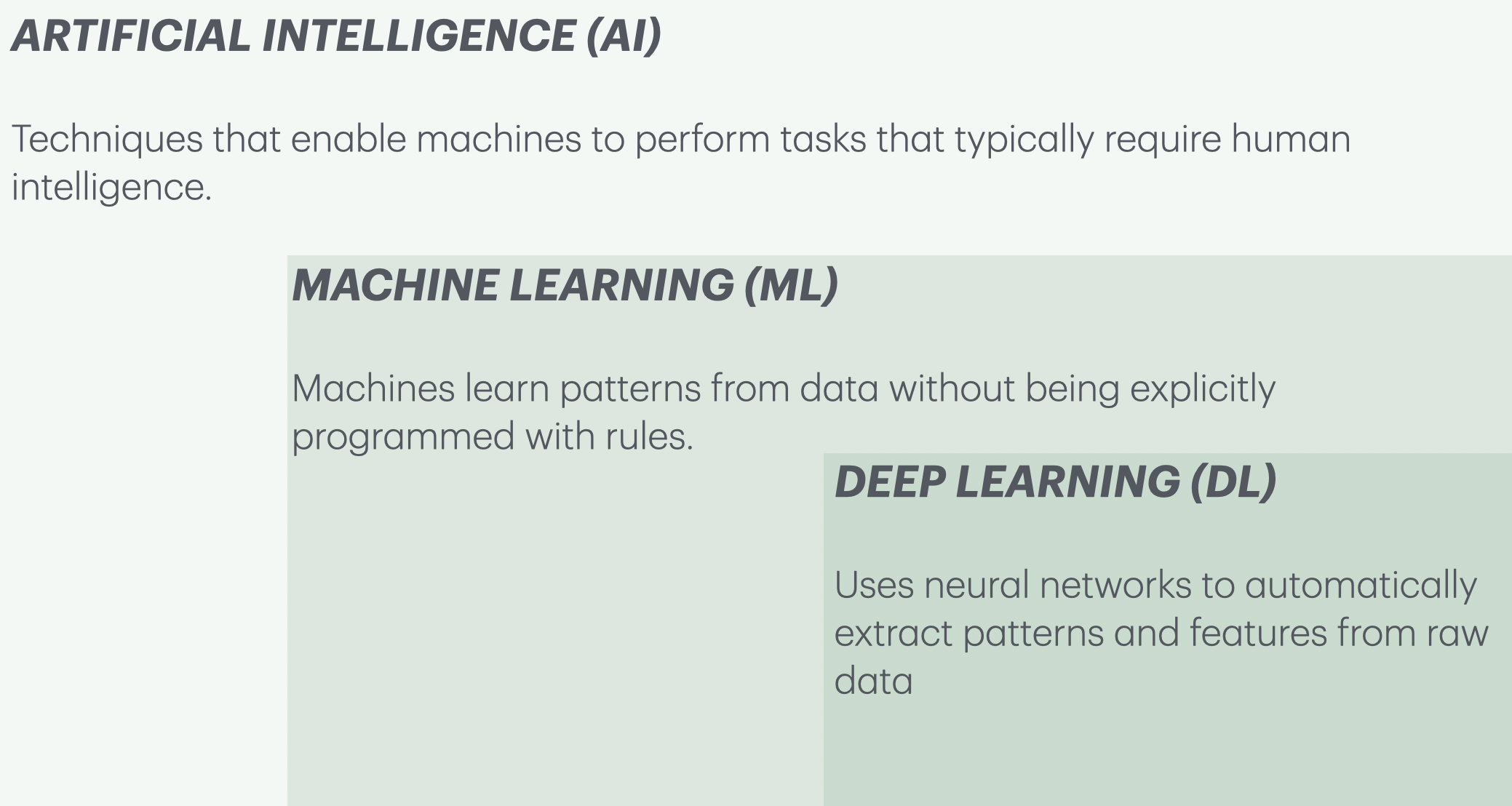
AI vs. ML vs. DL
- What is AI, and how does it relate to Machine Learning (ML) and Deep Learning (DL)?
 {.nostretch fig-align=“center” width=“700px”}
Image classification
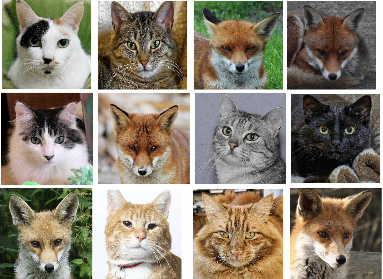
- Imagine you want to teach a robot to tell cats and foxes apart.
- How would you approach it?
AI approach: example
- You hard-code rules: “If the image has fur, whiskers, and pointy ears, it’s a cat.”
- This works for normal cases, but what if the cat is missing an ear? Or if the fox has short fur?
ML approach: example
- We don’t tell the model the exact rule. Instead, we give it labeled examples, and it learns which features matter most.
- small nose ✅
- round face ✅
- whiskers ✅
- Instead of giving rules, we let the model figure out the best combination of features from data.
DL approach: example
- The robot figures out the best features by itself using a neural network.
- Instead of humans selecting features, the neural network extracts them automatically, from edges to textures to full shapes.
- The more data it sees, the better it gets.
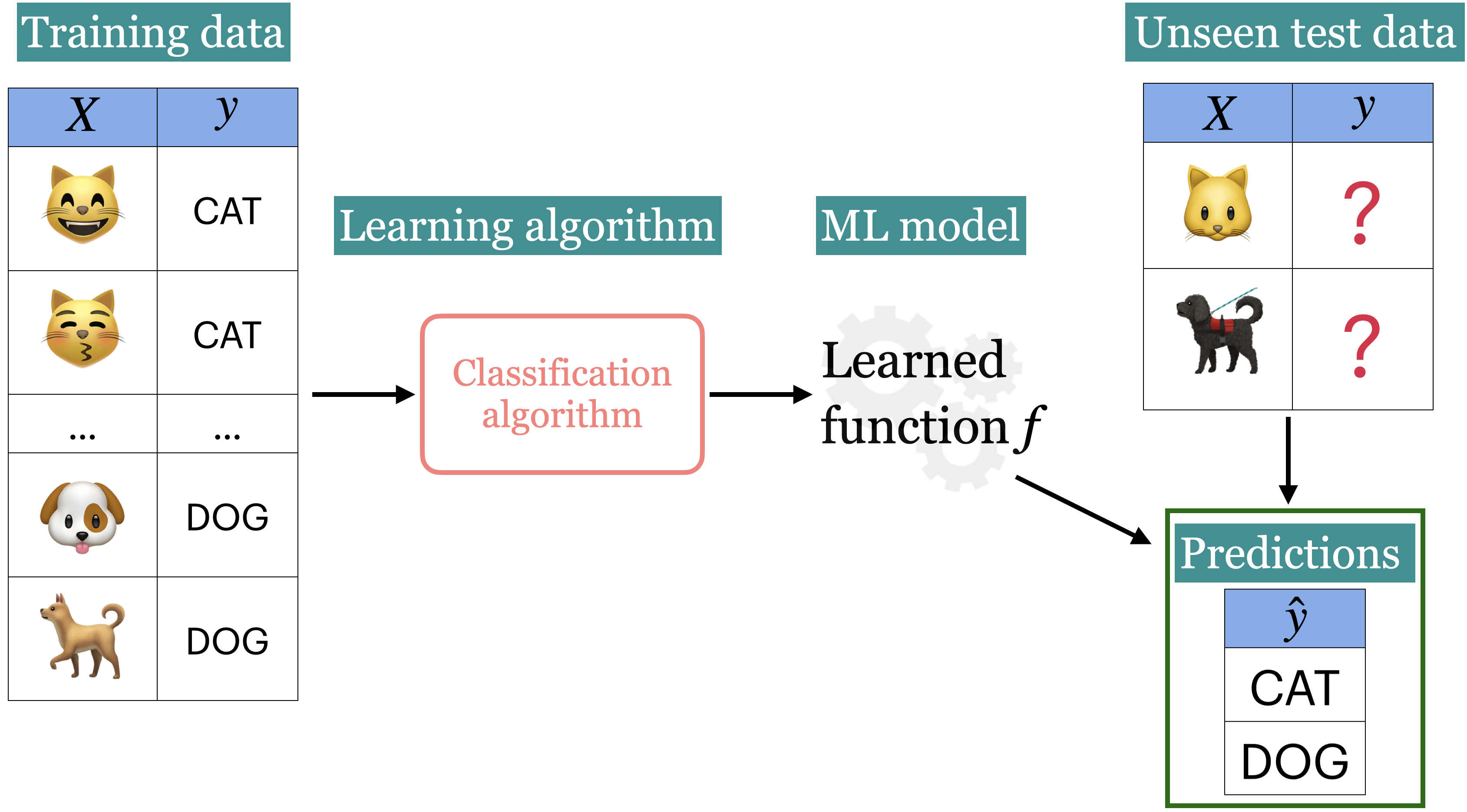
Supervised learning
- The most common type of machine learning is supervised learning.
- We aim to learn a function \(f\) that maps input features (\(X\)) to target values (\(y\)).
- Once trained, we use \(f(X)\) to make predictions on new, unseen data.
Terminology
Here are a few rows from the data.
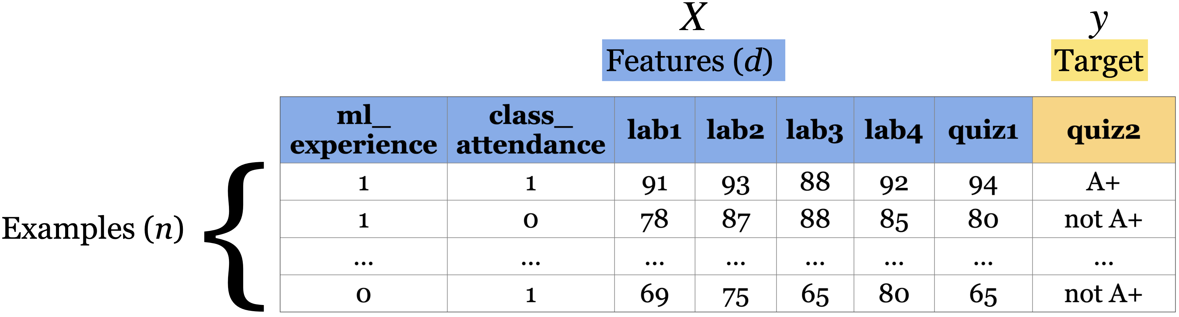
- Features: relevant characteristics of the problem, usually suggested by experts (typically denoted by \(X\)).
- Target: the variable we want to predict (typically denoted by \(y\)).
- Example: A row of feature values
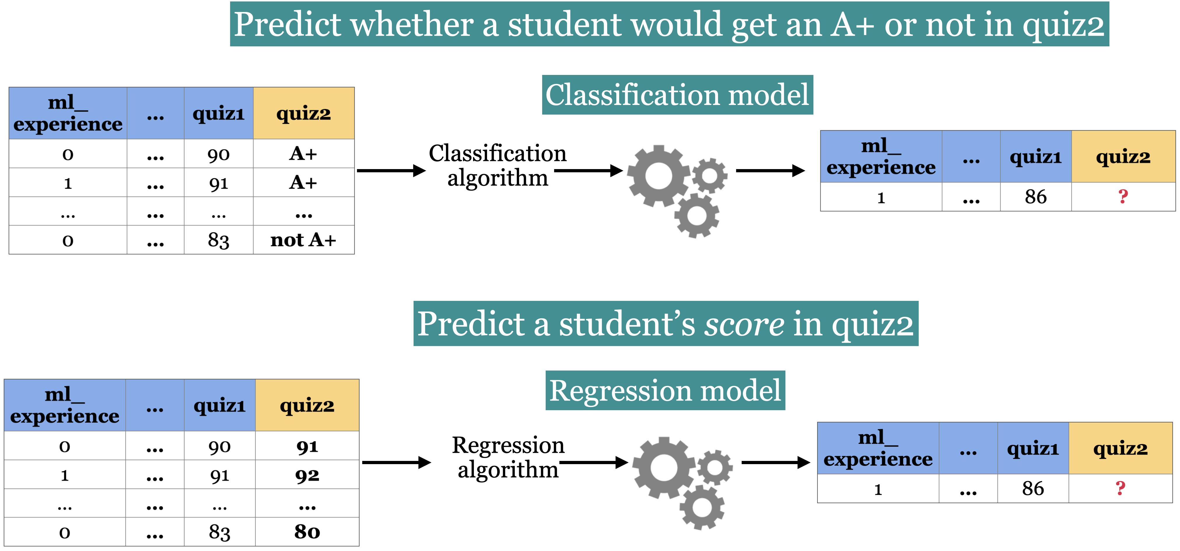
Classification vs. Regression
Linear models
- Linear models make an assumption that the relationship between
Xandyis linear. - In this case, with only one feature, our model is a straight line.
- What do we need to represent a line?
- Slope (\(w_1\)): Determines the angle of the line.
- Y-intercept (\(w_0\)): Where the line crosses the y-axis. This is also called the bias term
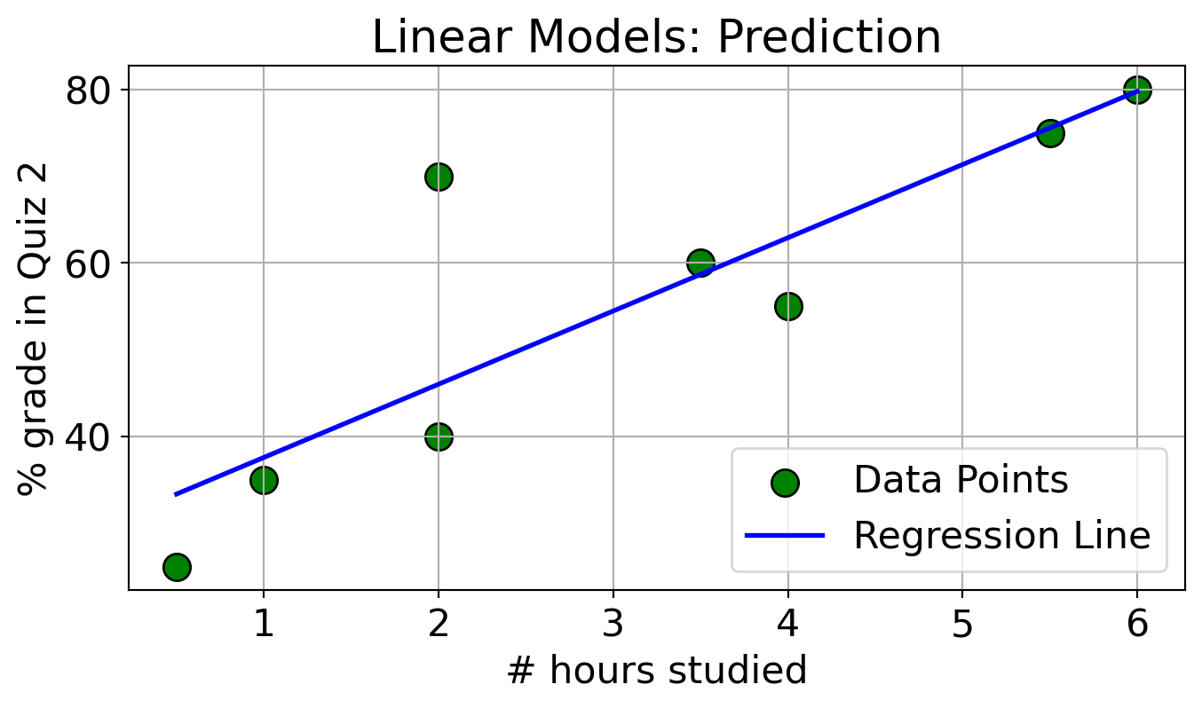
- Making predictions
- \(y_{hat} = w_1 \times \text{\# hours studied} + w_0\)
Logistic regression
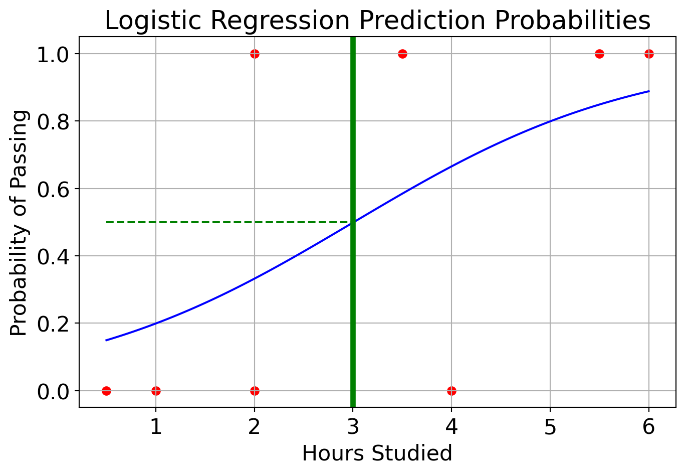
- Calculate the weighted sum \(z = w_1 \times \text{\# hours studied} + w_0\)
- Apply sigmoid function to get a number between 0 and 1.
- \(\hat{y} = \sigma(z) = \frac{1}{1 + e^{-z}}\)
- Model
- If you study \(\leq 3\) hours, you fail.
- If you study \(> 3\) hours, you pass.
A graphical view of a linear model

- We have 4 features: x[0], x[1], x[2], x[3]
- The output is calculated as \(y = x[0]w[0] + x[1]w[1] + x[2]w[2] + x[3]w[3]\)
- For simplicity, we are ignoring the bias term.
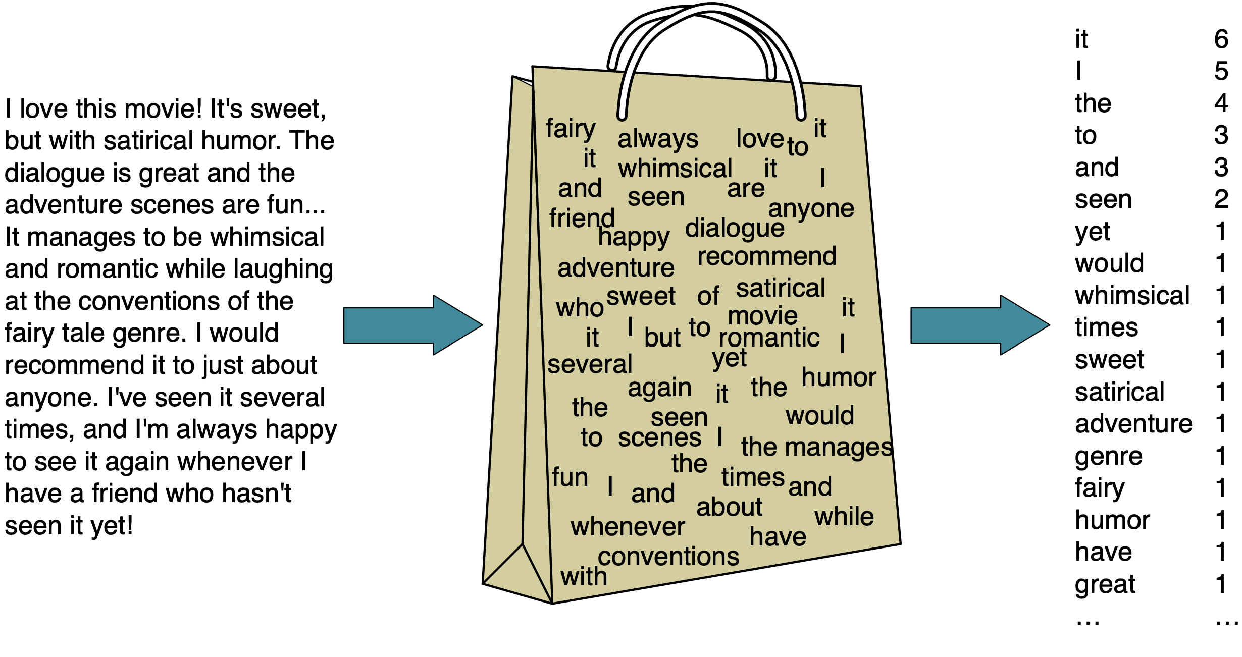
Bag of Words
- To create features that logistic regression can use, we will represent these reviews with a “bag of words” representation.
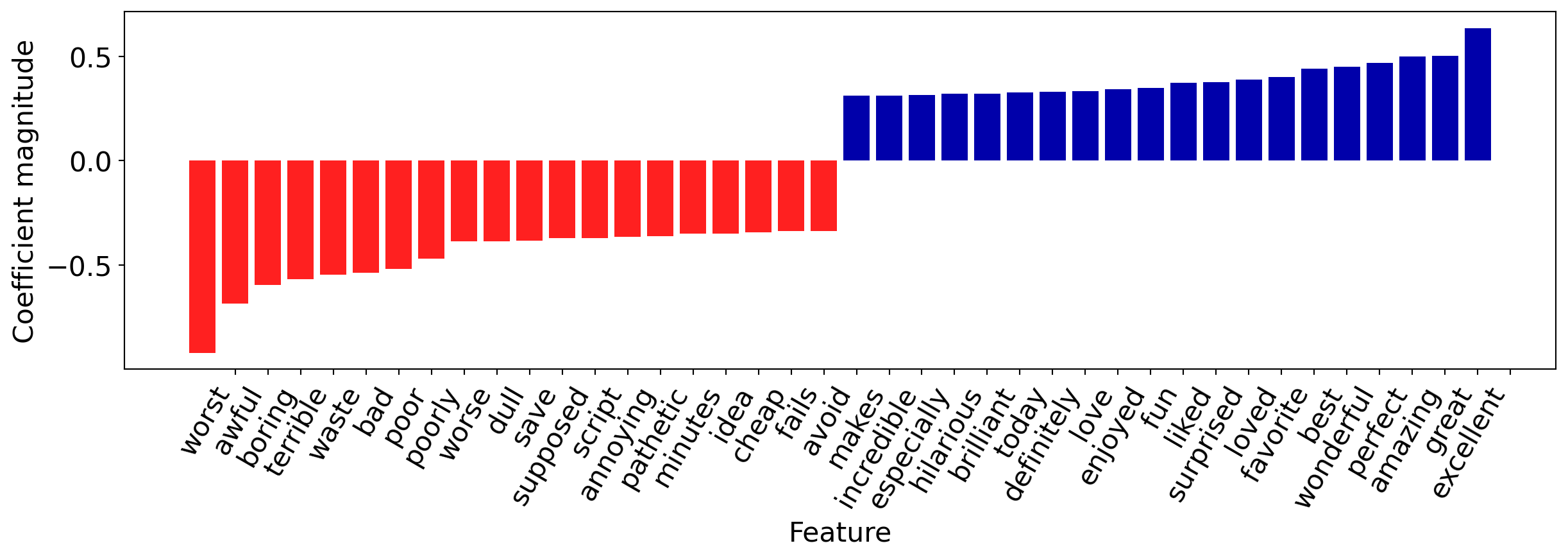
Investigating the model
Let’s visualize the 20 most important features.