CPSC 330 Lecture 11: Ensembles

Varada Kolhatkar

Focus on the breath!

Announcements

• Midterm next week. Important information about midterm 1
  • https://edstem.org/us/courses/104703/discussion/8335467
  • Good news for you: You’ll have access to our course notes and sklearn, pandas, and numpy documentation in the midterm!
• HW4 was due Monday, Oct 12 at 11:59 pm.
• HW5 is now available and due Oct 26 at 11:59 pm. This project brings together what you’ve learned. Start early!

Today’s big questions

1. When does combining models improve predictions?
2. How do random forests and boosting build and combine trees differently?
3. How do voting and stacking combine different model types, and when is the extra cost worthwhile?

iClicker Exercise 11.0

Which of the following scenarios has worked effectively for you in the past?

• 1. Working independently on a project/assignment
• 2. Working with like-minded people
• 3. Teaming up with a diverse group offering varied perspectives and skills

Use this as a discussion prompt, not a question with one correct answer. Diverse perspectives motivate the analogy, but model ensembles still need validation evidence.

The wisdom of crowds

Groups can make better decisions when members contribute useful, different perspectives.

Source

Can averaging help?

A house sells for $500,000.

Model	Predicted price
Linear model	$460,000
Decision tree	$520,000

• What is their average prediction?
• What if both models predicted $460,000?

The average is $490,000: an error of $10,000, smaller than either individual error. If both predict $460,000, averaging changes nothing. This is an illustration on one example, not evidence that the ensemble generalizes better.

Ensembles: The key idea

Training data fit three models; a new example passes through each model, and their predictions are combined by voting or averaging

Image created by GPT-6.1 Sol

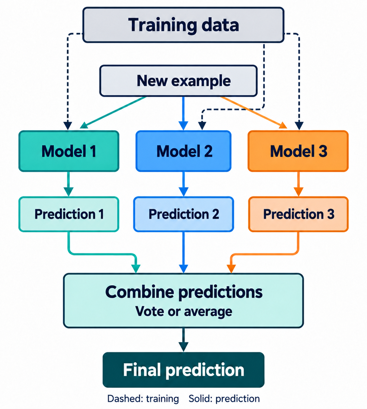
An ensemble combines predictions from multiple models.

• Classification: combine labels or class probabilities
• Regression: average numerical predictions

The aim is better predictions on new examples.

AI-generated redraw of the ensemble schematic, with separate training and prediction paths. Original conceptual reference: https://sebastianraschka.com/pdf/lecture-notes/stat451fs20/07-ensembles__slides.pdf

Same accuracy, different mistakes

In a binary classification problem, each model gets 2 of 3 correct. Which ensemble performs better?

✓ Correct and ✗ Wrong

Same mistakes

Example	Model 1	Model 2	Model 3	Majority vote
Example 1	✗	✗	✗	✗
Example 2	✓	✓	✓	✓
Example 3	✓	✓	✓	✓

Majority vote: 2/3 correct

Different mistakes

Example	Model 1	Model 2	Model 3	Majority vote
Example 1	✗	✓	✓	✓
Example 2	✓	✗	✓	✓
Example 3	✓	✓	✗	✓

Majority vote: 3/3 correct

All three examples have true class 1. A check means prediction 1; a cross means prediction 0. This shared true label makes majority voting on correctness equivalent to voting on class labels. Each base model has accuracy 2/3 in both tables. Ask students to calculate the vote before revealing the last column and results together. Complementary errors improve the vote in the second table. These three-row examples illustrate arithmetic, not generalization evidence. Adapted from the expertise–diversity examples in DSCI 573 notes.

Diversity alone isn’t enough

In a binary classification problem, each model gets 1 of 3 correct, on a different example. What does the majority vote predict?

✓ Correct and ✗ Wrong

Example	Model 1	Model 2	Model 3	Majority vote
Example 1	✓	✗	✗	✗
Example 2	✗	✓	✗	✗
Example 3	✗	✗	✓	✗

Majority vote: 0/3 correct: two wrong predictions outvote one correct prediction on every row.

All three examples again have true class 1; correct predictions are 1 and wrong predictions are 0. Diversity does not guarantee improvement: this particular hard vote is wrong on every example. Do not infer that weak models can never help an ensemble, or that every model must individually outperform chance. Evaluate the combination on held-out data. Adapted from DSCI 573 notes.

Useful predictions and different mistakes

• Expertise: individual models learn useful patterns
• Diversity: their errors can offset one another
• Identical predictions gain nothing from averaging

Use validation results to check whether combining models helps.

Today’s methods

• Random forests: train randomized trees independently, then average
• Gradient boosting: build trees sequentially to correct the current ensemble
• Voting and averaging: combine different types of models directly
• Stacking: learn a model that combines base predictions

Random forests

iClicker Exercise 11.1

What could we randomize to build a diverse collection of useful trees? Select all that seem promising.

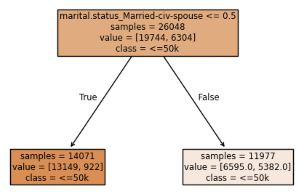
• 1. Which training rows each tree sees
• 2. Which features a split can use
• 3. The thresholds used for splits
• 4. The maximum depth of each tree
• 5. The target labels assigned to training examples

Use this as an exploratory poll before introducing how random forests work. A–D are plausible ways to create different trees; students do not need to know any named ensemble method. Randomizing depth is possible, although it is not a defining mechanism of standard random forests. E creates variation but destroys the input–target relationship we want to learn: diversity alone is not enough. Invite students to explain their choices, then introduce random forests’ two sources of randomness on the next slide. Random thresholds are also a valid idea, used in Extra Trees; do not mark C wrong simply because standard random forests use optimized thresholds.

Two sources of randomness

1. Bootstrap samples: each tree draws its own training rows, with replacement
2. Random feature subsets: each split considers a new random subset of features

Both encourage trees to make different predictions.

Building a training set for each tree

Original training rows: A B C D E F

Each ID represents a complete row: features and target.

1. Draw one row: select B
2. Put it back: all six rows remain available
3. Repeat six times: B B A E B D

	Training row IDs	Repeated IDs	Missing IDs
Tree 1	B B A E B D	B (3 times)	C, F
Tree 2	F C C A F D	C, F (twice each)	B, E

Each tree gets six rows; some repeat and others are absent.

Before revealing the table, ask which IDs repeat and which are missing from the first sample. The second sample is drawn independently from the original six rows, not from the first sample or from its omitted rows. Repeated IDs mean repeated copies of the same complete training row, not new observations. For a training set of n rows, the default bootstrap sample uses n draws with replacement; other sample sizes are possible. Different samples encourage different trees but do not guarantee distinct samples or predictions. Training models on bootstrap samples and aggregating their predictions is bagging: bootstrap aggregating. This slide illustrates the sampling step; random feature subsets provide the forest’s second source of randomness.

Random features at each split

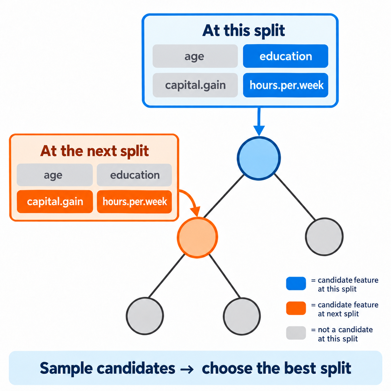
Random subsets of Adult census features: education and hours.per.week at one split, capital.gain and hours.per.week at the next

Image created by GPT-6.1 Sol

• Sample candidate features at each split
• Choose the best split among those candidates
• An excluded feature can be available at a later split

Why choose a new subset at each split instead of one subset per tree?

Suppose capital.gain is useful but excluded from the candidates at the first split.

• One subset per tree: when could that tree use the feature?
• A new subset per split: what changes?

With one fixed subset, the feature is unavailable throughout that tree. With fresh subsets, it may be available at later splits: capital.gain is grey at the first split and orange at the next in the preceding diagram. The diagram illustrates four features from Adult; actual subsets are sampled from all available transformed features. This preserves access to useful information while encouraging different trees. Neither strategy has a universally fixed level of diversity or predictive strength.

How a forest predicts

• Classification in scikit-learn: average the trees’ class probabilities; choose the class with the largest average
• Regression: average the trees’ numerical predictions

Trees are trained independently: no tree corrects an earlier tree.

RandomForestClassifier uses probability averaging, which can disagree with majority voting on class labels. Trace a row through the small forest in the chapter demo.

Random-forest hyperparameters

Hyperparameter	Controls
n_estimators	Number of trees in the average
max_depth	Maximum depth of each tree
min_samples_leaf	Minimum samples supporting a leaf
max_features	Candidate features considered at each split

Fewer candidate features encourage diversity but can weaken individual trees.

More trees versus deeper trees

• Deeper trees can fit finer details, including noise
• More trees stabilize the average from the same training procedure
• Gains from more trees often level off; computation and memory keep growing

Adding trees does not automatically fix a training–validation gap.

Validation scores need not improve monotonically as trees are added. Use cross-validation to investigate tree depth and leaf size as well as forest size. A forest can still overfit.

iClicker Exercise 11.2

Select the most accurate statement about a standard random forest.

• 1. Each tree independently draws a bootstrap sample of the training rows
• 2. Each tree is restricted to one randomly selected feature subset throughout training
• 3. Choose n_estimators using whichever value scores best on the reserved test set
• 4. Each tree learns to correct the predictions of the previous tree
• 5. Averaging cannot outperform the most accurate individual model

Answer: A. Independent draws need not produce distinct samples. B describes a fixed feature subset per tree, rather than per split. C uses test data for model selection. D describes the sequential idea of boosting. E is contradicted by complementary errors, as in the opening example.

Demo

Go to the Demo

• Trace a prediction through the small forest
• Compare the tree and forest on the same validation folds
• Inspect accuracy and fit time as the forest grows

Does the gain justify the extra computation?

Gradient boosting

Random forests and boosting

Random forests	Gradient boosting
Train trees independently	Train trees sequentially
Average predictions	Add learned corrections
Randomness encourages different trees	Each tree improves the current ensemble

Both require validation; neither guarantees better generalization.

Boosting example: One starting prediction

Predict house price from floor area, using squared-error loss. Prices are in thousands of dollars; these are invented training data.

Start by predicting the mean price, 280, for every house.

Floor area	Actual price	Starting prediction	Residual: actual − prediction
50	200	280	−80
70	220	280	−60
90	260	280	−20
110	300	280	+20
130	340	280	+60
150	360	280	+80

Where should we lower predictions? Where should we raise them?

Use the same six houses as the Chapter 11 notebook. The mean is (200 + 220 + 260 + 300 + 340 + 360)/6 = 280. Residual means actual minus current prediction: negative means we predicted too high; positive means we predicted too low. Point out that the smaller houses need downward corrections and the larger houses need upward corrections. This is a squared-error regression example; classification uses loss-dependent corrections to numerical scores, not subtraction of class labels.

Boosting example: Learn a correction

Fit a one-split tree: input = floor area; target = residual. It splits at floor area 100 and predicts each group’s mean residual.

Houses	Residuals	Tree’s correction
Area ≤ 100	−80, −60, −20	−53.3
Area > 100	+20, +60, +80	+53.3

With learning rate 0.5, apply half the correction:

Houses	Updated prediction
Area ≤ 100	280 − 26.7 = 253.3
Area > 100	280 + 26.7 = 306.7

Repeat: compute the remaining errors and fit the next correction tree.

The first stump in the notebook splits between areas 90 and 110. Its lower leaf predicts (−80 − 60 − 20)/3 = −53.333…; the upper leaf predicts +53.333…. The learning rate scales these corrections to ±26.666…. Values on the slide are rounded to one decimal; calculations use unrounded values. The first house now has prediction 253.3 instead of 280, so its residual becomes about −53.3 rather than −80. The 90-area house is now predicted slightly too low: the group correction need not improve every individual row, even though it reduces total squared error here. The next tree uses the original floor-area feature and the updated residuals of the entire ensemble. At prediction time, start at 280 and add the scaled outputs of all correction trees; do not average them. The notebook continues for a second round and predicts for a new house. These training calculations illustrate the algorithm; use held-out data to evaluate generalization.

Controlling boosting complexity

• Rounds: how many corrections we add
• Learning rate: how much of each correction we apply
• Tree size: how complex each correction can be

Tune these together using validation data.

More rounds can overfit; smaller steps may need more rounds.

Early stopping uses a validation score or loss to decide when to stop. This is model selection: never use the reserved test set. Within cross-validation, early-stopping data must come from the training portion of the fold. Boosting can also include random row or feature sampling.

Gradient-boosted tree implementations

Implementation	Useful distinction
scikit-learn	Classic and histogram-based implementations
XGBoost	Efficient tree building and explicit regularization
LightGBM	Histogram splits and leaf-wise tree growth
CatBoost	Built-in handling of categorical features

Compare on your task; no library is a universal winner.

These are emphases, not exclusive capabilities. In the notes’ common encoded-data comparison, CatBoost does not use its native categorical handling. Keep library-specific options and code in the notebook.

Demo: Compare boosting candidates

Use the same training data, validation folds, and metric.

• Compare against the single tree and random forest
• Read validation scores alongside fold-to-fold variation
• Compare fit and prediction costs

A small score difference may not justify a much slower model.

Voting, averaging, and stacking

Combining different model types

For example: logistic regression + random forest + boosted trees.

• Classification: combine labels or probabilities
• Regression: average numerical predictions
• Different model types can encourage complementary errors

Check the combination against its strongest individual model.

Hard and soft voting

Hard voting

• Combine predicted labels
• Choose the class with the most votes

Soft voting

• Average class probabilities
• Choose the class with the largest average

VotingClassifier supports both methods. VotingRegressor averages numerical predictions. Equal weighting is a starting point; selecting weights is also a model-selection decision.

Can hard and soft voting disagree?

Three binary classifiers predict these positive-class probabilities:

Model A	Model B	Model C
0.51	0.51	0.01

• Which class wins the hard vote at a 0.5 threshold?
• Which class wins the soft vote?
• Is using probabilities always better?

Hard voting selects positive, two votes to one. The mean probability is 1.03/3 ≈ 0.343, so soft voting selects negative. An inaccurate, overconfident model can distort probability averages. Validate the choice rather than assuming soft voting wins.

Stacking: Learn the combination

Base predictions become features for a meta-model.

Illustrative training inputs: each model supplies \(P(\text{income} > 50K)\).

	Logistic regression	Random forest	LGBM	Target
0	0.34	0.40	0.10	≤50K
1	0.72	0.65	0.85	>50K
2	0.48	0.55	0.30	≤50K
3	0.20	0.65	0.80	>50K

• Inputs: the three probability columns, using out-of-fold predictions
• Target: the original income label; index is only a row identifier
• For a new row, the meta-model predicts from the base probabilities

The values are illustrative, not measured results. LGBM denotes LightGBM. Every probability refers to the same positive class, income >50K; a value of 0.34 means a predicted probability of 34% for that class, even when the observed target is ≤50K. Each training row’s probabilities must come from base pipelines fitted without that row, including preprocessing. Neither the index nor the target is an input feature. For binary classification, one class probability per base model suffices. A logistic-regression meta-model learns a combination beyond a simple average; its coefficients are not accuracy rankings or percentages of trust.

Train the meta-model on held-out predictions

1. Split the training data into folds
2. Fit each base pipeline on the other folds; predict the held-out fold
3. Repeat until every training row has out-of-fold predictions
4. Fit the meta-model on those predictions and the training labels

Each row’s inputs come from base models fitted without that row.

Refit base pipelines on all training data. For a new row, pass their predictions to the trained meta-model.

Do not train the meta-model on in-sample predictions from base models fitted on all those same rows: overfitting can give it an unrealistically favourable view of the models. Keep learned preprocessing inside every base pipeline.

Evaluating the whole stack

• Evaluate the complete training procedure on held-out data
• Keep evaluation rows out of base-model and meta-model fitting
• Compare with voting and the strongest individual candidate

Stacking adds fitting cost; improvement is not guaranteed.

With outer cross-validation, each outer training portion has its own internal folds for generating meta-model inputs. The outer validation portion evaluates the complete fitted stack. Do not precompute a single out-of-fold table on all training data and then cross-validate just the meta-model: some base fits would have seen labels from the evaluation fold. Keep the reserved test set out of all selection decisions.

Demo: Does combining models help?

• Compare voting and stacking with their constituent models
• Inspect their probability calculations and validation results
• Weigh any gain against training, prediction, and maintenance costs

Keep the ensemble only when the evidence supports it.

Comparing ensemble methods

Method	Training	Prediction
Random forest	Independent randomized trees	Average probabilities or numbers
Gradient boosting	Successive correction trees	Add scaled corrections
Voting / averaging	Separate base models	Vote or average
Stacking	Base models + meta-model trained on held-out predictions	Pass base predictions to meta-model

All have classification and regression versions.

Key takeaways

• Useful, complementary predictions make ensembles promising
• More forest trees stabilize an average; more boosting rounds add corrections
• Stacking needs held-out base predictions for meta-model training
• Choose using validation performance and practical cost

Ensembles class demo

Existing class demo notebook