CPSC 330 Lecture 17: Introduction to computer vision

Varada Kolhatkar

Focus on the breath!

Announcements

• HW7 has been released (a new homework on transfer learning)
• No classes or OH during the midterm break.
• Midterm 2 coming up next week!
• If you find the breathing exercises helpful, you’re very welcome to join our weekly meditation sessions.
  • 🕑 When? Every Tuesday at 1 PM
  • 📍 Where? ICCS 146

iClicker: shopping recommendations for Eva

A shop uses content-based filtering with backpack attributes: Waterproof, Laptop compartment, and Recycled material. Eva has rated 12 backpacks.

How should the shop predict Eva’s rating for a new backpack?

• (A) Fit Ridge using the 12 backpacks’ attributes and Eva’s ratings, then pass the new backpack’s attributes to that model.
• (B) Fit Ridge using other shoppers’ ratings as features and Eva’s ratings as targets.
• (C) Fit Ridge using backpack attributes and all shoppers’ ratings together, without identifying the shoppers.
• (D) Recommend only backpacks Eva has already rated because a new backpack has no rating.

Correct answer: A.

Use Eva’s training ratings only. X has 12 rows (backpacks) and three columns (attributes). y contains Eva’s 12 corresponding ratings. Fit a separate Ridge model for Eva, then supply the new backpack’s three attributes in the same column order to predict her rating.

B uses other shoppers’ rating patterns rather than product attributes, moving toward collaborative filtering. C pools different shoppers’ preferences without representing whose rating we want to predict. D misses the benefit of content features: a new item can receive a prediction even without ratings, provided its attributes are available and Eva already has a fitted model. A shopper without training ratings would need a fallback.

Numerical follow-up: Suppose Eva’s fitted coefficients for Waterproof, Laptop compartment, and Recycled material are (0.8, -0.4, 0.6), with intercept 3.0. What rating does her model predict for a backpack with attributes (1, 0, 1)?

\[\hat r_{\mathrm{Eva},j}=3.0+1(0.8)+0(-0.4)+1(0.6)=4.4.\]

These are hypothetical fitted values. Eva’s model learns three feature coefficients and an intercept. The number of training backpacks determines the number of rows, not the number of coefficients. Coefficients describe associations in Eva’s ratings, not causal effects on enjoyment.

Today’s big questions

1. How do neural networks learn useful features?
2. Why do CNNs use local, shared filters for images?
3. How can a pretrained model help us classify new labels?
4. How do we evaluate the resulting classifier?

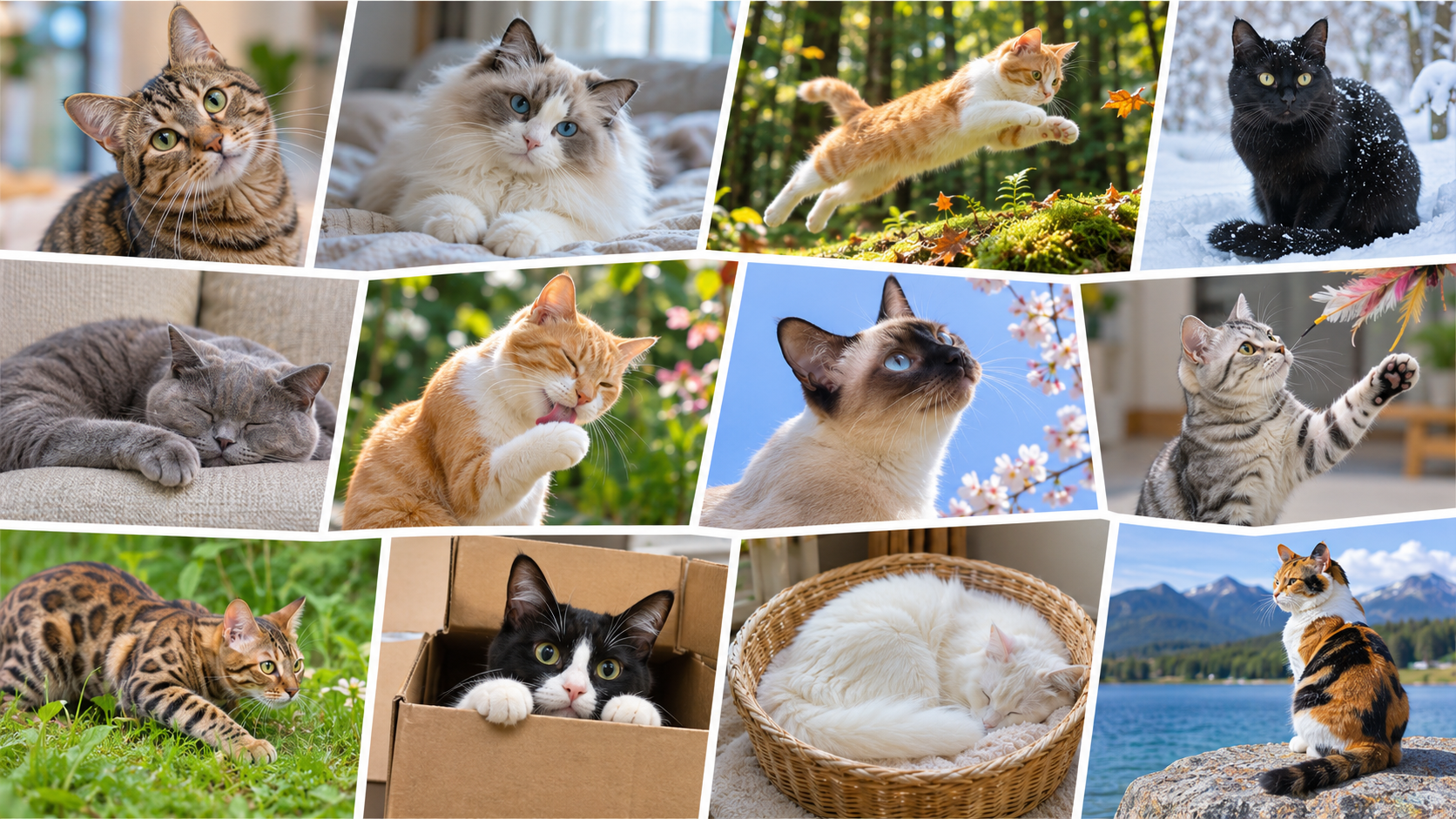
One label, many appearances

Cats with different appearances, poses, and backgrounds

Which differences matter for the label cat?

Pause and ask: “What changes across these pictures, and what stays the same?” Invite a few observations: coat colour and pattern, pose, viewpoint, lighting, and background vary, but every image still has the label cat.

To a computer, these images are arrays of numbers. Two cat images can have very different pixel values. Even moving the same cat within an image changes which pixels contain its ears, eyes, or fur. Recognizing a cat therefore requires more than matching an exact pixel pattern.

Ask: “Would coat colour change our answer?” For cat classification, usually no. If our task were to classify coat colours, it would matter. Which differences we want a model to tolerate depends on the target label.

A useful image representation should retain evidence that helps distinguish cats from other categories while tolerating variation within the cat category. We will use neural networks to produce learned features rather than try to list every useful visual feature ourselves. This does not guarantee that the model ignores backgrounds or other shortcuts, so representative evaluation images still matter.

Transition: “What model from our current toolbox would you try for image classification? What features would you give it?” Invite students to connect this task to familiar supervised-learning methods before introducing CNNs.

Image classification with our current toolbox

What model would you try for image classification?

What features would you give it?

Think about logistic regression, KNN, or random forests.

Allow a brief discussion. Several familiar classifiers can accept numerical image features. Ask students what one row of X would contain and what y would represent.

Pixel values are one possible starting point. Connect back to the cat images: changes in pose, lighting, or background can change many pixels without changing the label. The choice of representation matters as well as the choice of classifier.

CNNs for image classification

A convolutional neural network (CNN) is a neural network architecture designed to work with images.

• We will build high-level intuition for how CNNs work.
• We can use pretrained CNNs for our own tasks without studying every architectural or training detail.

Let’s begin with a brief introduction to neural networks.

CNNs are a common approach to image classification. Their layers learn useful image features from training examples, reducing the need to hand-design those features.

We will not derive the full architecture or train a CNN from scratch. Our practical goal is to use a pretrained model and understand enough of the workflow to apply it appropriately.

Before discussing what makes a CNN suited to images, introduce the neural-network idea using a model students already know: logistic regression.

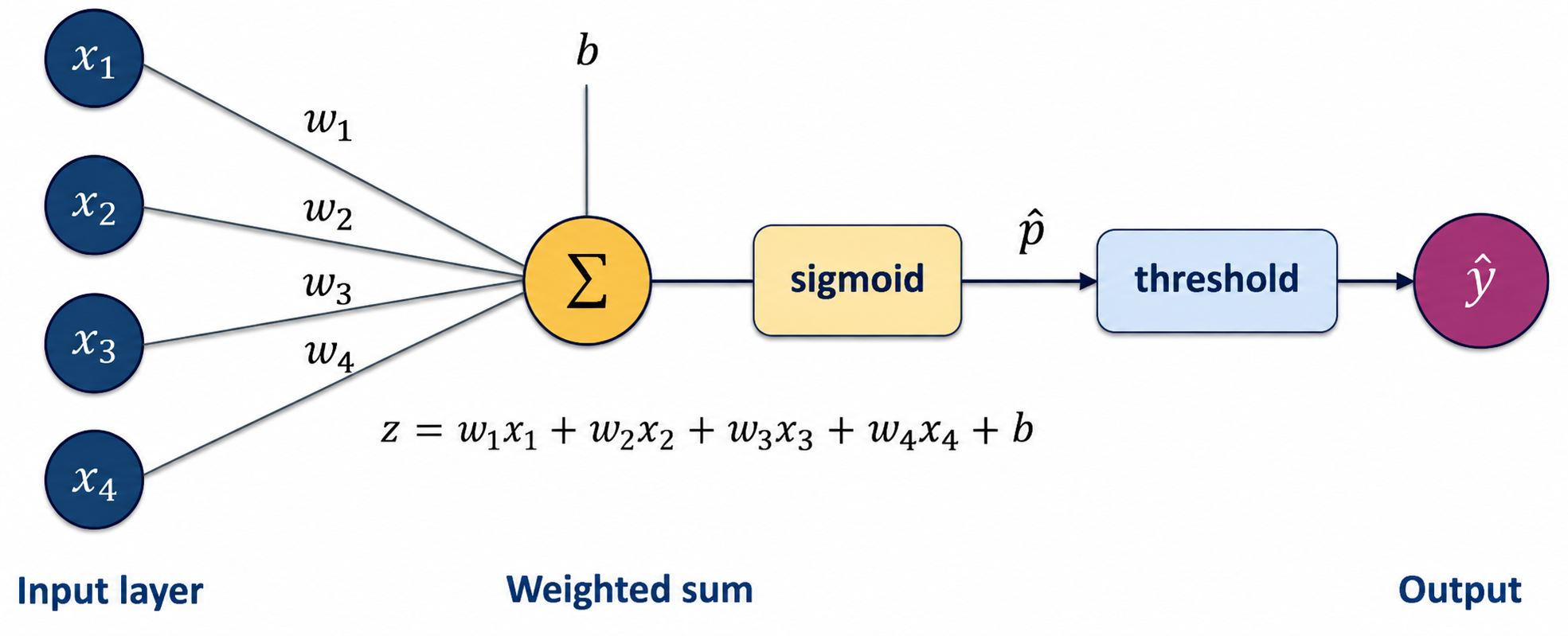
A graphical view of logistic regression

Four inputs, weighted sum and bias, sigmoid, and threshold

• Weights and an intercept produce a score.
• Sigmoid converts the score into a binary class probability.
• A threshold converts that probability into a label.

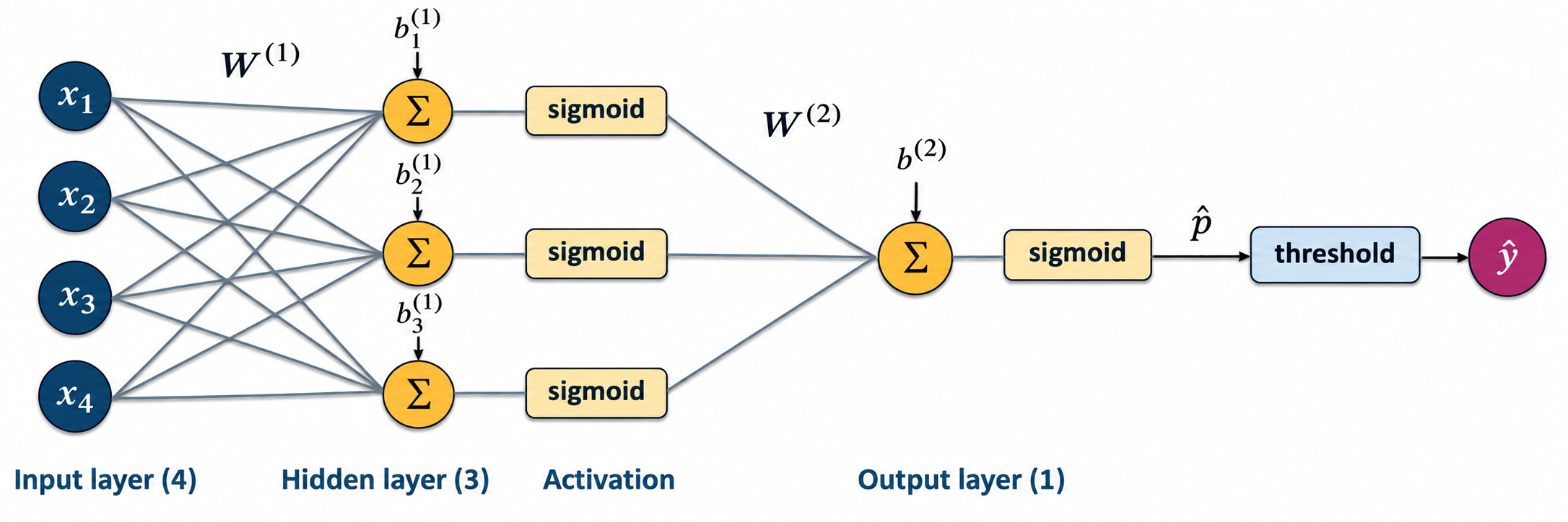
A neural network with one hidden layer

Four inputs, three nonlinear hidden units, and a binary output

Each hidden unit computes its own weighted sum and bias, then applies a nonlinear activation. Its output becomes a feature for the next layer.

How many parameters do we learn?

Four inputs, three nonlinear hidden units, and a binary output

With 4 inputs, 3 hidden units, and 1 output unit:

• How many weights do we learn?
• How many biases do we learn?

Give students a moment to count. Ask them to distinguish connections (weights) from units with an intercept (biases).

Input to hidden layer: each of the three hidden units receives four inputs, giving 4 × 3 = 12 weights and 3 biases.

Hidden layer to output: the output unit receives three hidden features, giving 3 × 1 = 3 weights and 1 bias.

Total: 15 weights and 4 biases, or 19 learned parameters.

The input nodes simply supply feature values, so they have no learned biases. Each hidden unit and the output unit has one bias. The sigmoid activation and threshold add no learned parameters here.

Compare with logistic regression on the same four inputs: 4 weights and 1 bias, or 5 parameters. Adding the hidden layer introduces intermediate learned features and increases the parameter count.

Computing the first hidden feature

Four inputs, three nonlinear hidden units, and a binary output

\[ \begin{aligned} z_1^{(1)} &= w_{11}^{(1)}x_1 + w_{12}^{(1)}x_2 + w_{13}^{(1)}x_3 + w_{14}^{(1)}x_4 + b_1^{(1)} \\ h_1 &= \operatorname{sigmoid}\!\left(z_1^{(1)}\right) \end{aligned} \]

• Superscript \((1)\) identifies the first layer, not a power.
• \(w_{12}^{(1)}\) connects input 2 to hidden unit 1.
• Repeat with different weights and biases to obtain \(h_2\) and \(h_3\).

Trace the four incoming connections to the first hidden unit in the diagram. Each input is multiplied by its own weight. Add these contributions and the unit’s bias to obtain its score, z_1^(1). Apply sigmoid to obtain h_1.

In w_12^(1), the first subscript identifies the receiving hidden unit and the second identifies the input. The superscript identifies the layer. The bias also belongs to this specific hidden unit.

The other hidden units receive the same four inputs but use their own weights and biases. Their outputs can therefore represent different transformations of those inputs. We now have three learned features, h_1, h_2, and h_3. We do not threshold them.

Computing the output

Four inputs, three nonlinear hidden units, and a binary output

\[ \begin{aligned} z^{(2)} &= w_1^{(2)}h_1 + w_2^{(2)}h_2 + w_3^{(2)}h_3 + b^{(2)} \\ \hat p &= \operatorname{sigmoid}\!\left(z^{(2)}\right) \end{aligned} \]

• Layer \((2)\) combines the three hidden features using its own weights and bias.
• \(\hat p\) is the predicted probability of the positive class.
• Computing the hidden features and prediction is a forward pass.

Trace the three connections from the hidden units to the output unit. This is the same weighted-sum-and-sigmoid computation as binary logistic regression, now using h_1, h_2, and h_3 as inputs instead of the original features.

The superscript (2) identifies the output layer. Since there is only one output unit, we use one subscript on each output weight to identify its incoming hidden feature.

Distinguish the roles of the sigmoid outputs: the hidden outputs are learned features, while the final output is the predicted probability of the positive class. With a decision threshold of 0.5, predict class 1 when p-hat is at least 0.5 and class 0 otherwise. Thresholding is the final decision step, not part of computing the hidden features.

A forward pass uses the current parameter values without updating them. Training is what adjusts the weights and biases.

Why nonlinear activations?

Stacking weighted sums without nonlinear activations still gives a linear model.

• Nonlinear hidden activations allow nonlinear decision boundaries.
• ReLU is another activation: \(\operatorname{ReLU}(z)=\max(0,z)\).
• Multiple hidden layers repeatedly transform the representation.

This is the idea behind deep learning.

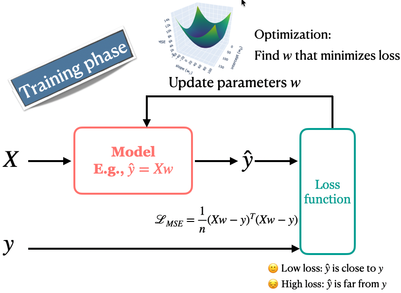
How does a network learn?

Supervised learning uses labelled examples to fit a model

A loss measures disagreement with known targets. Training adjusts weights to reduce that loss.

We’ll use a pretrained model with fixed weights to extract image features, then train a familiar model, such as logistic regression, on those features.

Introduction to computer vision

Computer vision tasks

Classification, localization, object detection, and instance segmentation

Today we focus on image classification: one category for an entire image.

Images as numerical arrays

• Grayscale: height × width intensity values.
• RGB: height × width × 3 colour channels.
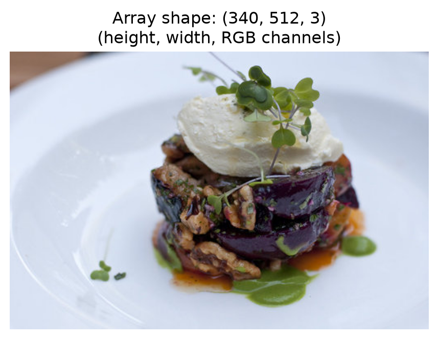
• A 340 × 512 RGB image has 522,240 values.

Why use local image structure?

Flattening preserves pixel values, but an ordinary classifier does not automatically use the fact that nearby pixels form patterns.

• Moving an object can change many input values.
• Connecting every pixel to every hidden unit creates many parameters.
• A CNN uses local filters and shares their weights across locations.

Convolutions and shared filters

A filter moves across an input array to produce a feature map

A filter computes a weighted sum over a local patch. Reusing it across locations produces a feature map.

Explore image kernels

Convolutional neural networks

Convolutions, ReLU, pooling, and a classification head

Convolutions and activations build features. Pooling reduces spatial dimensions. A classification head maps features to scores.

Figure reused from the book chapter. Original source: Google Developers, https://developers.google.com/machine-learning.

Pretrained CNNs

Why start with a pretrained model?

Training a CNN from scratch can require substantial labelled data, computing power, and time.

Companies and research groups have already trained models on large image datasets.

A pretrained model gives us a starting point: an architecture with weights already learned from data.

Connect to the CNN diagram: the filter weights and classification weights all have to be learned during training. For large models, doing this from scratch can be expensive, particularly when we have little labelled data for our own task.

We can reuse weights that another team has already learned and released. Loading the architecture alone would give us a network structure, but pretrained weights supply the learned parameter values.

Pretraining does not guarantee success on a new task. Its usefulness depends on the source data, our target images, and how we evaluate the resulting workflow.

Three ways to use a pretrained model

1. Use it directly: predict its original categories with its weights fixed.
2. Extract features: keep the pretrained weights fixed and train a new classifier, such as logistic regression, on its features.
3. Fine-tune it: update some or all pretrained weights using our task’s training data.

We’ll focus on direct prediction and frozen feature extraction.

For direct prediction, retain the original classification head and label vocabulary. This is useful when those labels answer our question.

For frozen feature extraction, take the representation before the original classification head. Keep the CNN fixed and fit a new classifier for our own labels. The scaler and logistic regression learn from our training data, while the CNN does not.

For fine-tuning, training changes some or all of the pretrained network’s weights. This requires additional modelling choices and computation, and it can overfit a small dataset. We will not implement it in this course.

Transition: First, inspect what a pretrained ImageNet classifier can predict without any additional training. Later, reuse its features for a new classification task.

ImageNet classification

• We use MobileNet V3 Small, trained for 1,000 ImageNet categories.
• Its original classifier chooses among those categories.
• It cannot invent a new output label.

Multiclass classification: each example receives one of several labels. Multilabel classification allows several labels per example.

Imagenet classes

weights = models.MobileNet_V3_Small_Weights.IMAGENET1K_V1
imagenet_model = models.mobilenet_v3_small(weights=weights).eval()
imagenet_preprocess = weights.transforms()
imagenet_labels = weights.meta["categories"]
imagenet_labels[700:715]

['paper towel',
 'parachute',
 'parallel bars',
 'park bench',
 'parking meter',
 'passenger car',
 'patio',
 'pay-phone',
 'pedestal',
 'pencil box',
 'pencil sharpener',
 'perfume',
 'Petri dish',
 'photocopier',
 'pick']

Multinomial logistic regression

• Binary: one score, converted into the positive-class probability using sigmoid.
• Multinomial: one score per class, each computed using that class’s own coefficients and intercept.
• Softmax converts those scores into class probabilities that sum to one.

Predict the class with the highest probability.

A CNN’s classification head applies the same score-to-probability idea to learned image features.

Recall that a binary logistic regression score is a weighted sum of features plus an intercept. For multinomial logistic regression, repeat that computation with a separate set of coefficients and an intercept for each class.

The scores can be negative and do not sum to one. Softmax converts the whole set of scores into a probability distribution over the available classes. We choose one class, so this is multiclass rather than multilabel classification.

A CNN’s feature extractor is more complex than logistic regression, but its output can follow this same pattern: one score per class followed by softmax. The next slide illustrates this with four classes instead of ImageNet’s 1,000.

Softmax probabilities

Suppose a classifier produces these scores for four classes:

import pandas as pd
scores = torch.tensor([1.2, -0.4, 2.0, 0.7])
probabilities = torch.softmax(scores, dim=0)
pd.DataFrame({
    "Class": [0, 1, 2, 3],
    "Score": scores.numpy(),
    "Probability": probabilities.numpy(),
}).round(3)

	Class	Score	Probability
0	0	1.2	0.248
1	1	-0.4	0.050
2	2	2.0	0.552
3	3	0.7	0.150

Class 2 wins: it has the highest score and probability.

Softmax preserves the score ordering. A high probability does not guarantee a correct prediction.

Read across a row to connect each score to its probability. The unrounded probabilities sum to one. Displayed values may differ slightly from one when summed because of rounding.

Class labels here are numbered from zero, so class 2 is the third row. Softmax preserves the ordering of the scores, so we could identify the winning class directly from its score. Softmax also gives a probability distribution over all four classes.

These probabilities are relative to the available labels. A model still assigns them when an image does not belong to any useful category in its vocabulary. Return to this limitation when inspecting pretrained predictions.

Softmax

For scores \(z_1,\ldots,z_K\),

\[P(y=k)=\frac{e^{z_k}}{\sum_{j=1}^{K}e^{z_j}}.\]

Exponentiation makes values positive. Dividing by their sum makes probabilities add to one.

Every probability depends on all class scores.

Using pretrained models out of the box

• We reuse an image classifier trained elsewhere to predict labels for new photos.
• The model learned from labeled images during its original training; we do not train it here.

Class demo

When the labels do not answer our question

Suppose our task is to identify UBC landmarks.

The model predicts an ImageNet category with high confidence.

• Does confidence establish that the landmark is correct?
• Can the model predict a landmark absent from its output vocabulary?
• How could we adapt it to our own labels?

Frozen feature extraction

Use the pretrained CNN to produce a representation for each image.

1. Apply the preprocessing expected by the pretrained weights.
2. Remove the original classification head.
3. Keep the CNN weights fixed.
4. Train a scaler and logistic regression for our food labels.

Our seven labels can differ from ImageNet’s labels.

Food classification: live demo

Class demo

Image preprocessing versus feature scaling

Operation	What it does	Where its settings come from
Image preprocessing	Resize, crop, normalize RGB input	Pretrained weight specification
Feature extraction	Produce 576 learned features	Frozen ImageNet weights
Feature scaling	Learn feature means and scales	Current training rows
Logistic regression	Learn food class coefficients	Training features and labels

Keep scaling inside the scikit-learn pipeline.

The classifier always chooses a known food category, even for an unrelated image. One prediction does not measure accuracy.

What learns from our labels?

We extract frozen ImageNet features from 300 plant photographs and train a classifier for five species.

1. Which components learned from ImageNet? Which learn from the plants?
2. Must the species appear in ImageNet’s original labels?
3. If we change only C, must we run the CNN again?
4. What if we change the image preprocessing?

The CNN stays fixed. The scaler learns training feature statistics, and logistic regression learns coefficients and intercepts. The species need not match ImageNet labels. Changing C reuses features. Changing preprocessing requires new features.

Connection to HW7

Food demo	HW7
Seven food categories	Six waste categories
Fixed training/validation folders	Training data with stratified CV, reserved test set
Dummy versus pretrained features	Also compare low-resolution pixel features
One logistic regression setting	Choose C using GridSearchCV
Validation mistakes	Final test metrics and application limits

Both use frozen MobileNet features and a scaler inside the pipeline.

The Golden Rule still applies

• Fit scaling and logistic regression using only the current fitting rows.
• Use validation data or CV to choose settings.
• Evaluate the selected workflow once on the reserved test set.
• Keep related images, such as frames from the same video, together when splitting.

Extracting deterministic frozen features does not fit to held-out images. Using their results to choose settings does.

Practical limitations

• Domain shift: features from everyday photos may transfer poorly to other image conditions.
• Pretrained models inherit gaps and biases from their source data.
• Larger extractors cost more time and memory.
• Fine-tuning updates CNN weights on the new data. It is outside our scope and may overfit a small dataset.

Evaluate on images representative of the intended use.

Summary

• Neural networks combine weighted sums and nonlinear activations to learn features.
• CNNs use local filters shared across image locations.
• Pretrained predictions use the original label vocabulary.
• Frozen feature extraction supports new labels with a familiar classifier.
• Compare baselines, inspect errors, and protect the data splits.